
2022-09-16 Differentiation
Contents
2022-09-16 Differentiation#
Last time#
Newton’s method for systems
Bratu nonlinear PDE
p-Laplacian
Today#
NLsolve Newton solver library
p-Laplacian robustness
diagnostics
Algorithmic differentiation via Zygote
Symbolic differentiation
Structured by-hand differentiation
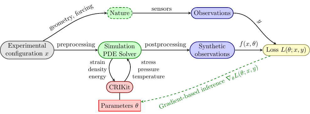
Concept of PDE-based inference (inverse problems)
using Plots
default(linewidth=3)
using LinearAlgebra
using SparseArrays

function vander(x, k=nothing)
    if k === nothing
        k = length(x)
    end
    V = ones(length(x), k)
    for j = 2:k
        V[:, j] = V[:, j-1] .* x
    end
    V
end

function fdstencil(source, target, k)
    "kth derivative stencil from source to target"
    x = source .- target
    V = vander(x)
    rhs = zero(x)'
    rhs[k+1] = factorial(k)
    rhs / V
end

function my_spy(A)
    cmax = norm(vec(A), Inf)
    s = max(1, ceil(120 / size(A, 1)))
    spy(A, marker=(:square, s), c=:diverging_rainbow_bgymr_45_85_c67_n256, clims=(-cmax, cmax))
end


function advdiff_sparse(n, kappa, wind, forcing)
    x = LinRange(-1, 1, n)
    xstag = (x[1:end-1] + x[2:end]) / 2
    rhs = forcing.(x)
    kappa_stag = kappa.(xstag)
    rows = [1, n]
    cols = [1, n]
    vals = [1., 1.] # diagonals entries (float)
    rhs[[1,n]] .= 0 # boundary condition
    for i in 2:n-1
        flux_L = -kappa_stag[i-1] * fdstencil(x[i-1:i], xstag[i-1], 1) +
            wind * (wind > 0 ? [1 0] : [0 1])
        flux_R = -kappa_stag[i] * fdstencil(x[i:i+1], xstag[i], 1) +
            wind * (wind > 0 ? [1 0] : [0 1])
        weights = fdstencil(xstag[i-1:i], x[i], 1)
        append!(rows, [i,i,i])
        append!(cols, i-1:i+1)
        append!(vals, weights[1] *  [flux_L..., 0] + weights[2] * [0, flux_R...])
    end
    L = sparse(rows, cols, vals)
    x, L, rhs
end

function newton(residual, jacobian, u0; maxits=20)
    u = u0
    uhist = [copy(u)]
    normhist = []
    for k in 1:maxits
        f = residual(u)
        push!(normhist, norm(f))
        J = jacobian(u)
        delta_u = - J \ f
        u += delta_u
        push!(uhist, copy(u))
    end
    uhist, normhist
end
newton (generic function with 1 method)
\(p\)-Laplacian#
plaplace_p = 1.5
plaplace_forcing = 0.
function plaplace_f(u)
    n = length(u)
    h = 2 / (n - 1)
    u = copy(u)
    f = copy(u)
    u[[1, n]] = [0, 1]
    f[n] -= 1
    for i in 2:n-1
        u_xstag = diff(u[i-1:i+1]) / h
        kappa_stag = abs.(u_xstag) .^ (plaplace_p - 2)
        f[i] = [1/h, -1/h]' *
            (kappa_stag .* u_xstag) - plaplace_forcing
    end
    f
end
plaplace_f (generic function with 1 method)
function plaplace_J(u)
    n = length(u)
    h = 2 / (n - 1)
    u = copy(u)
    u[[1, n]] = [0, 1]
    rows = [1, n]
    cols = [1, n]
    vals = [1., 1.] # diagonals entries (float)
    for i in 2:n-1
        js = i-1:i+1
        u_xstag = diff(u[js]) / h
        kappa_stag = abs.(u_xstag) .^ (plaplace_p - 2)
        fi = [h, -h]' * (kappa_stag .* u_xstag)
        fi_ujs = [-kappa_stag[1]/h^2,
                  sum(kappa_stag)/h^2,
                  -kappa_stag[2]/h^2]
        mask = 1 .< js .< n
        append!(rows, [i,i,i][mask])
        append!(cols, js[mask])
        append!(vals, fi_ujs[mask])
    end
    sparse(rows, cols, vals)
end
plaplace_J (generic function with 1 method)
Try solving#
n = 20
x = collect(LinRange(-1., 1, n))
u0 = (1 .+ x) / 2

plaplace_p = 1.3 # try different values
plaplace_forcing = 1
uhist, normhist = newton(plaplace_f, plaplace_J, u0; maxits=20);
plot(normhist, marker=:circle, yscale=:log10, ylims=(1e-10, 1e3))

plot(x, uhist[1:5:end], marker=:auto, legend=:bottomright)

What’s wrong?#
Using Zygote to differentiate#
using Zygote

gradient(x -> x^2, 3)
(6.0,)
function plaplace_fpoint(u, h)
    u_xstag = diff(u) / h
    kappa_stag = abs.(u_xstag) .^ (plaplace_p - 2)
    [1/h, -1/h]' * (kappa_stag .* u_xstag)
end

gradient(u -> plaplace_fpoint(u, .1), [0., .7, 1.])
([-7.683385553661419, 21.58727725682051, -13.903891703159092],)
p-Laplacian with Zygote#
function plaplace_fzygote(u)
    n = length(u)
    h = 2 / (n - 1)
    u = copy(u)
    f = copy(u)
    u[[1, n]] = [0, 1]
    f[n] -= 1
    for i in 2:n-1
        f[i] = plaplace_fpoint(u[i-1:i+1], h) - plaplace_forcing
    end
    f
end
plaplace_fzygote (generic function with 1 method)
function plaplace_Jzygote(u)
    n = length(u)
    h = 2 / (n - 1)
    u = copy(u)
    u[[1, n]] = [0, 1]
    rows = [1, n]
    cols = [1, n]
    vals = [1., 1.] # diagonals entries (float)
    for i in 2:n-1
        js = i-1:i+1
        fi_ujs = gradient(ujs -> plaplace_fpoint(ujs, h), u[js])[1]
        mask = 1 .< js .< n
        append!(rows, [i,i,i][mask])
        append!(cols, js[mask])
        append!(vals, fi_ujs[mask])
    end
    sparse(rows, cols, vals)
end
plaplace_Jzygote (generic function with 1 method)
Experiment with parameters#
plaplace_p = 1.4
plaplace_forcing = 1
u0 = (x .+ 1)
uhist, normhist = newton(plaplace_fzygote, plaplace_Jzygote, u0; maxits=10);
plot(normhist, marker=:auto, yscale=:log10)

plot(x, uhist, marker=:auto, legend=:topleft)

Can you fix the
plaplace_Jto differentiate correctly (analytically)?What is causing Newton to diverge?
How might we fix or work around it?
A model problem for Newton divergence; compare NLsolve#
k = 1. # what happens as this is changed
fk(x) = tanh.(k*x)
Jk(x) = reshape(k / cosh.(k*x).^2, 1, 1)
xhist, normhist = newton(fk, Jk, [2.], maxits=10)
plot(xhist, fk.(xhist), marker=:circle, legend=:bottomright)
plot!(fk, xlims=(-20, 2), linewidth=1)

using NLsolve

nlsolve(x -> fk(x) .+ .5, Jk, [5.], show_trace=true)
Iter     f(x) inf-norm    Step 2-norm
------   --------------   --------------
     0     1.499909e+00              NaN
     1     5.000000e-01     5.000000e+00
     2     3.788284e-02     5.000000e-01
     3     8.529212e-04     4.816956e-02
     4     4.836986e-07     1.135938e-03
     5     1.559863e-13     6.449311e-07
Results of Nonlinear Solver Algorithm
 * Algorithm: Trust-region with dogleg and autoscaling
 * Starting Point: [5.0]
 * Zero: [-0.5493061443338468]
 * Inf-norm of residuals: 0.000000
 * Iterations: 5
 * Convergence: true
   * |x - x'| < 0.0e+00: false
   * |f(x)| < 1.0e-08: true
 * Function Calls (f): 6
 * Jacobian Calls (df/dx): 6
NLsolve for p-Laplacian#
plaplace_p = 1.5
plaplace_forcing = 1
u0 = (x .+ 1) / 2
sol = nlsolve(plaplace_fzygote, plaplace_Jzygote, u0,
    store_trace=true)
plaplace_p = 1.3
sol = nlsolve(plaplace_fzygote, plaplace_Jzygote, sol.zero,
    store_trace=true)
fnorms = [sol.trace[i].fnorm for i in 1:sol.iterations]
plot(fnorms, marker=:circle, yscale=:log10)

plot(x, [sol.initial_x sol.zero], label=["initial" "solution"])

What about symbolic differentiation?#
import Symbolics: Differential, expand_derivatives, @variables
@variables x
Dx = Differential(x)
y = tanh(k*x)
Dx(y)
expand_derivatives(Dx(y))
Cool, what about composition of functions#
y = x
for _ in 1:2
    y = cos(y^pi) * log(y)
end
expand_derivatives(Dx(y))
The size of these expressions can grow exponentially.
Hand coding derivatives: it’s all chain rule and associativity#
function f(x)
    y = x
    for _ in 1:2
        a = y^pi
        b = cos(a)
        c = log(y)
        y = b * c
    end
    y
end

f(1.9), gradient(f, 1.9)
(-1.5346823414986814, (-34.03241959914049,))
function df(x, dx)
    y = x
    dy = dx
    for _ in 1:2
        a = y^pi
        da = pi * y^(pi-1) * dy
        b = cos(a)
        db = -sin(a) * da
        c = log(y)
        dc = 1/y * dy
        y = b * c
        dy = db * c + b * dc
    end
    dy
end

df(1.9, 1)
-34.03241959914048
We can go the other way#
We can differentiate a composition \(h(g(f(x)))\) as
What we’ve done above is called “forward mode”, and amounts to placing the parentheses in the chain rule like
The expression means the same thing if we rearrange the parentheses,
which we can compute with in reverse order via
A reverse mode example#
function g(x)
    a = x^pi
    b = cos(a)
    c = log(x)
    y = b * c
    y
end
(g(1.4), gradient(g, 1.4))
(-0.32484122107701546, (-1.2559761698835525,))
function gback(x, y_)
    a = x^pi
    b = cos(a)
    c = log(x)
    y = b * c
    # backward pass
    c_ = y_ * b
    b_ = c * y_
    a_ = -sin(a) * b_
    x_ = 1/x * c_ + pi * x^(pi-1) * a_
    x_
end
gback(1.4, 1)
-1.2559761698835525
Kinds of algorithmic differentation#
Source transformation: Fortran code in, Fortran code out
Duplicates compiler features, usually incomplete language coverage
Produces efficient code
Operator overloading: C++ types
Hard to vectorize
Loops are effectively unrolled/inefficient
Just-in-time compilation: tightly coupled with compiler
JIT lag
Needs dynamic language features (JAX) or tight integration with compiler (Zygote, Enzyme)
Some sharp bits
How does Zygote work?#
h1(x) = x^3 + 3*x
h2(x) = ((x * x)  + 3) * x
@code_llvm h1(4.)
;  @ In[144]:1 within `h1`
define double @julia_h1_18050(double %0) #0 {
top:
; ┌ @ intfuncs.jl:322 within `literal_pow`
; │┌ @ operators.jl:591 within `*` @ float.jl:385
    %1 = fmul double %0, %0
    %2 = fmul double %1, %0
; └└
; ┌ @ promotion.jl:389 within `*` @ float.jl:385
   %3 = fmul double %0, 3.000000e+00
; └
; ┌ @ float.jl:383 within `+`
   %4 = fadd double %3, %2
; └
  ret double %4
}
@code_llvm gradient(h1, 4.)
;  @ /home/jed/.julia/packages/Zygote/xGkZ5/src/compiler/interface.jl:95 within `gradient`
define [1 x double] @julia_gradient_15323(double %0) #0 {
top:
;  @ /home/jed/.julia/packages/Zygote/xGkZ5/src/compiler/interface.jl:97 within `gradient`
; ┌ @ /home/jed/.julia/packages/Zygote/xGkZ5/src/compiler/interface.jl:45 within `#60`
; │┌ @ In[54]:1 within `Pullback`
; ││┌ @ /home/jed/.julia/packages/Zygote/xGkZ5/src/compiler/chainrules.jl:206 within `ZBack`
; │││┌ @ /home/jed/.julia/packages/Zygote/xGkZ5/src/lib/number.jl:12 within `literal_pow_pullback`
; ││││┌ @ intfuncs.jl:321 within `literal_pow`
; │││││┌ @ float.jl:385 within `*`
        %1 = fmul double %0, %0
; ││││└└
; ││││┌ @ promotion.jl:389 within `*` @ float.jl:385
       %2 = fmul double %1, 3.000000e+00
; │└└└└
; │┌ @ /home/jed/.julia/packages/Zygote/xGkZ5/src/lib/lib.jl:17 within `accum`
; ││┌ @ float.jl:383 within `+`
     %3 = fadd double %2, 3.000000e+00
; └└└
;  @ /home/jed/.julia/packages/Zygote/xGkZ5/src/compiler/interface.jl:98 within `gradient`
  %.fca.0.insert = insertvalue [1 x double] zeroinitializer, double %3, 0
  ret [1 x double] %.fca.0.insert
}
Forward or reverse?#
It all depends on the shape.
One input, many outputs: use forward mode
“One input” can be looking in one direction
Many inputs, one output: use reverse mode
Will need to traverse execution backwards (“tape”)
Hierarchical checkpointing
About square? Forward is usually a bit more efficient.
Inference using PDE-based models#
Compressible Blasius boundary layer#
Activity will solve this 1D nonlinear PDE