2022-10-03 2D Advection-diffusion and waves#

Last time#

Implicit Runge-Kutta methods
Exploring/discussing tradeoffs
SciML benchmarks suite (DifferentialEquations.jl)

Today#

FD methods in 2D
Cost profile
The need for fast algebraic solvers
Wave equation and Hamiltonians
Symplectic integrators

using Plots
default(linewidth=3)
using LinearAlgebra
using SparseArrays

function my_spy(A)
    cmax = norm(vec(A), Inf)
    s = max(1, ceil(120 / size(A, 1)))
    spy(A, marker=(:square, s), c=:diverging_rainbow_bgymr_45_85_c67_n256, clims=(-cmax, cmax))
end
    
function plot_stability(Rz, title; xlims=(-2, 2), ylims=(-2, 2))
    x = LinRange(xlims[1], xlims[2], 100)
    y = LinRange(ylims[1], ylims[2], 100)
    heatmap(x, y, (x, y) -> abs(Rz(x + 1im*y)), c=:bwr, clims=(0, 2), aspect_ratio=:equal, title=title)
end

struct RKTable
    A::Matrix
    b::Vector
    c::Vector
    function RKTable(A, b)
        s = length(b)
        A = reshape(A, s, s)
        c = vec(sum(A, dims=2))
        new(A, b, c)
    end
end

function rk_stability(z, rk)
    s = length(rk.b)
    1 + z * rk.b' * ((I - z*rk.A) \ ones(s))
end

rk4 = RKTable([0 0 0 0; .5 0 0 0; 0 .5 0 0; 0 0 1 0], [1, 2, 2, 1] / 6)

function ode_rk_explicit(f, u0; tfinal=1., h=0.1, table=rk4)
    u = copy(u0)
    t = 0.
    n, s = length(u), length(table.c)
    fY = zeros(n, s)
    thist = [t]
    uhist = [u0]
    while t < tfinal
        tnext = min(t+h, tfinal)
        h = tnext - t
        for i in 1:s
            ti = t + h * table.c[i]
            Yi = u + h * sum(fY[:,1:i-1] * table.A[i,1:i-1], dims=2)
            fY[:,i] = f(ti, Yi)
        end
        u += h * fY * table.b
        t = tnext
        push!(thist, t)
        push!(uhist, u)
    end
    thist, hcat(uhist...)
end

ode_rk_explicit (generic function with 1 method)

Extending advection-diffusion to 2D#

1 dimension#

(20)#\[\begin{align} u_t + (- \kappa u_x + w u)_x &= f(x) & \text{ on } \Omega &= (a,b) \\ u(a) &= g_D(a) & u'(b) &= g_N(b) \end{align}\]

Cell Peclet number \(\mathrm{Pe}_h = \frac{\lvert w \rvert h}{\kappa}\)
- \(\mathrm{Pe}_h \lesssim 1\) avoids oscillations
- \(\mathrm{Pe}_h \gtrsim 1\) is non-stiff for time-dependent model
Centered versus upwind for advection
Need uniformly bounded \(\kappa \ge \epsilon > 0\)
“Strong form” not defined at discontinuities in \(\kappa\)
- Works okay using divergence form and fluxes at staggered points

2 dimensions#

(21)#\[\begin{align} u_t + \nabla\cdot\big(- \kappa \nabla u + \mathbf{w} u \big) &= f(x,y) & \text{ on } \Omega & \subset \mathbb R^2 \\ u|_{\Gamma_D} &= g_D(x,y) \\ (-\kappa \nabla u + \mathbf w u) \cdot \hat n|_{\Gamma_N} &= g_N(x,y) \end{align}\]

\(\Omega\) is some well-connected open set (we will assume simply connected) and the Dirichlet boundary \(\Gamma_D \subset \partial \Omega\) is nonempty.
Finite difference methods don’t have an elegant/flexible way to specify boundaries
We’ll choose \(\Omega = (-1, 1) \times (-1, 1)\)

On finite difference grids#

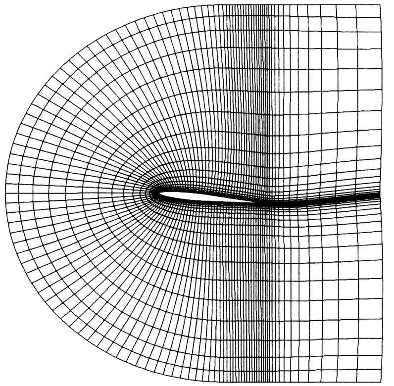
Non-uniform grids can mesh “special” domains
- Rare in 3D; overset grids, immersed boundary methods
Concept of staggering is complicated/ambiguous

Wesseling 11.4: A boundary-fitted grid around an airfoil.

Time-independent advection-diffusion#

Advection#

\[ \nabla\cdot(\mathbf w u) = \mathbf w \cdot \nabla u + (\nabla\cdot \mathbf w) u\]

If we choose divergence-free \(\mathbf w\), we can use the stencil

\[\begin{split} \mathbf w \cdot \nabla u \approx \frac 1 h \begin{bmatrix} & w_2 & \\ -w_1 & & w_1 \\ & -w_2 & \end{bmatrix} \!:\! \begin{bmatrix} u_{i-1, j+1} & u_{i, j+1} & u_{i+1,j+1} \\ u_{i-1, j} & u_{i, j} & u_{i+1,j} \\ u_{i-1, j-1} & u_{i, j-1} & u_{i+1,j-1} \\ \end{bmatrix} \end{split}\]

Diffusion#

\[ -\nabla\cdot(\kappa \nabla u) = -\kappa \nabla\cdot \nabla u - \nabla\kappa\cdot \nabla u\]

When would you trust this decomposition?
If we have constant \(\kappa\), we can write
\[\begin{split} -\kappa \nabla\cdot \nabla u \approx \frac{\kappa}{h^2} \begin{bmatrix} & -1 & \\ -1 & 4 & -1 \\ & -1 & \end{bmatrix} \!:\! \begin{bmatrix} u_{i-1, j+1} & u_{i, j+1} & u_{i+1,j+1} \\ u_{i-1, j} & u_{i, j} & u_{i+1,j} \\ u_{i-1, j-1} & u_{i, j-1} & u_{i+1,j-1} \\ \end{bmatrix} \end{split}\]

Advection-diffusion in code#

function advdiff_matrix(n; kappa=1, wind=[1, 1]/sqrt(2))
    h = 2 / n
    rows = Vector{Int64}()
    cols = Vector{Int64}()
    vals = Vector{Float64}()
    idx(i, j) = (i-1)*n + j
    stencil_advect = [-wind[1], -wind[2], 0, wind[1], wind[2]] / h
    stencil_diffuse = [-1, -1, 4, -1, -1] * kappa / h^2
    for i in 1:n
        for j in 1:n
            if i in [1, n] || j in [1, n]
                push!(rows, idx(i, j))
                push!(cols, idx(i, j))
                push!(vals, 1.)
            else
                append!(rows, repeat([idx(i,j)], 5))
                append!(cols, [idx(i-1,j), idx(i,j-1), idx(i,j), idx(i+1,j), idx(i,j+1)])
                append!(vals, stencil_advect + stencil_diffuse)
            end
        end
    end
    sparse(rows, cols, vals)
end

advdiff_matrix (generic function with 1 method)

Spy the matrix#

A = advdiff_matrix(6, wind=[1, 0], kappa=.001)
my_spy(A)

A = advdiff_matrix(20, wind=[2, 1], kappa=.1)
ev = eigvals(Matrix(-A))
scatter(real(ev), imag(ev))
scatter!([0], [0], color=:black, label=:none, marker=:plus)

Plot a solution#

n = 50
x = LinRange(-1, 1, n)
y = x
f = cos.(pi*x/2) * cos.(pi*y/2)'
heatmap(x, y, f, aspect_ratio=:equal)

A = advdiff_matrix(n, wind=[2,1], kappa=.001)
u = A \ vec(f)
heatmap(x, y, reshape(u, n, n), aspect_ratio=:equal)

What happens when advection dominates?
As you refine the grid?

Cost breadown and optimization#

using ProfileSVG
function assemble_and_solve(n)
    A = advdiff_matrix(n)
    x = LinRange(-1, 1, n)
    f = cos.(pi*x/2) * cos.(pi*x/2)'
    u = A \ vec(f)
end

@profview assemble_and_solve(400)

┌ Warning: The depth of this graph is 96, exceeding the `maxdepth` (=50).
│ The deeper frames will be truncated.
└ @ ProfileSVG /home/jed/.julia/packages/ProfileSVG/ecSyU/src/ProfileSVG.jl:275
┌ Warning: The depth of this graph is 96, exceeding the `maxdepth` (=50).
│ The deeper frames will be truncated.
└ @ ProfileSVG /home/jed/.julia/packages/ProfileSVG/ecSyU/src/ProfileSVG.jl:275

What’s left?#

Symmetric Dirichlet boundary conditions
Symmetric Neumann boundary conditions
Verification with method of manufactured solutions
Non-uniform grids
Upwinding for advection-dominated problems
Variable coefficients
Time-dependent problems
Fast algebraic solvers

Gas equations of state#

There are many ways to describe a gas

Name	variable	units
pressure	\(p\)	force/area
density	\(\rho\)	mass/volume
temperature	\(T\)	Kelvin
(specific) internal energy	\(e\)	energy/mass
entropy	\(s\)	energy/Kelvin

Equation of state#

\[ \rho, e \mapsto p, T \]

Ideal gas#

(22)#\[\begin{align} p &= \rho R T & e &= e(T) \end{align}\]

\[ p = (\gamma - 1) \rho e \]

pressure(rho, T) = rho*T

contour(LinRange(0, 2, 30), LinRange(0, 2, 30), pressure, xlabel="\$\\rho\$", ylabel="\$T\$")

Conservation equations#

Mass#

Let \(\mathbf u\) be the fluid velocity. The mass flux (mass/time) moving through an area \(A\) is

\[ \int_A \rho \mathbf u \cdot \hat{\mathbf n} .\]

If mass is conserved in a volume \(V\) with surface \(A\), then the total mass inside the volume must evolve as

\[ \int_V \rho_t = \left( \int_V \rho \right)_t = - \underbrace{\int_A \rho\mathbf u \cdot \hat{\mathbf n}}_{\int_V \nabla\cdot (\rho\mathbf u)},\]

where we have applied the divergence theorem. Dropping the integrals over arbitrary volumes, we have the evolution equation for conservation of mass.

\[ \rho_t + \nabla\cdot (\rho \mathbf u) = 0 \]

Momentum#

The momentum \(\rho \mathbf u\) has a flux that includes

convection \(\rho \mathbf u \otimes \mathbf u\)
- this is saying that each component of momentum is carried along in the vector velocity field
pressure \(p I\)
viscous \(-\boldsymbol\tau\)

A similar integral principle leads to the momentum equation

\[ (\rho \mathbf u)_t + \nabla\cdot\big[ \rho \mathbf u \otimes \mathbf u + p I - \boldsymbol \tau \big] = 0 \]

Numerical Solution of Partial Differential Equations

2022-10-03 2D Advection-diffusion and waves

Contents