.ipynb .pdf

repository open issue

Binder Live Code

Contents

2021-10-01 Runge-Kutta methods

Last time

• Stability for advection-diffusion

• Cost scaling

Today

• Accuracy and stability barriers

• Runge-Kutta methods

using Plots
using LinearAlgebra
using SparseArrays
using Zygote

function vander(x, k=nothing)
    if k === nothing
        k = length(x)
    end
    V = ones(length(x), k)
    for j = 2:k
        V[:, j] = V[:, j-1] .* x
    end
    V
end

function fdstencil(source, target, k)
    "kth derivative stencil from source to target"
    x = source .- target
    V = vander(x)
    rhs = zero(x)'
    rhs[k+1] = factorial(k)
    rhs / V
end

function newton(residual, jacobian, u0; maxits=20)
    u = u0
    uhist = [copy(u)]
    normhist = []
    for k in 1:maxits
        f = residual(u)
        push!(normhist, norm(f))
        J = jacobian(u)
        delta_u = - J \ f
        u += delta_u
        push!(uhist, copy(u))
    end
    uhist, normhist
end

function plot_stability(Rz, title; xlims=(-6, 2), ylims=(-4, 4))
    x = LinRange(xlims[1], xlims[2], 100)
    y = LinRange(ylims[1], ylims[2], 100)
    heatmap(x, y, (x, y) -> abs(Rz(x + 1im*y)), c=:bwr, clims=(0, 2), aspect_ratio=:equal, title=title)
end
Rz_theta(z, theta) = (1 + (1 - theta)*z) / (1 - theta*z)
plot_stability(z -> Rz_theta(z, .5), "Midpoint method")

function ode_theta_linear(A, u0; forcing=zero, tfinal=1, h=0.1, theta=.5)
    u = copy(u0)
    t = 0.
    thist = [t]
    uhist = [u0]
    while t < tfinal
        tnext = min(t+h, tfinal)
        h = tnext - t
        rhs = (I + h*(1-theta)*A) * u .+ h*forcing(t+h*theta)
        u = (I - h*theta*A) \ rhs
        t = tnext
        push!(thist, t)
        push!(uhist, u)
    end
    thist, hcat(uhist...)
end

function advdiff_matrix(n; kappa=1, wind=1, upwind=0.)
    dx = 2 / n
    rows = [1]
    cols = [1]
    vals = [0.]
    wrap(j) = (j + n - 1) % n + 1
    for i in 1:n
        append!(rows, [i, i, i])
        append!(cols, wrap.(i-1:i+1))
        diffuse = [-1, 2, -1] * kappa / dx^2
        advect_upwind = [-1, 1, 0] * wind / dx
        advect_center = [-1, 0, 1] * wind / 2dx
        stencil = -diffuse - upwind * advect_upwind - (1 - upwind) * advect_center
        append!(vals, stencil)
    end
    sparse(rows, cols, vals)
end
advdiff_matrix(5, kappa=.1)

5×5 SparseMatrixCSC{Float64, Int64} with 15 stored entries:
 -1.25   -0.625    ⋅       ⋅      1.875
  1.875  -1.25   -0.625    ⋅       ⋅ 
   ⋅      1.875  -1.25   -0.625    ⋅ 
   ⋅       ⋅      1.875  -1.25   -0.625
 -0.625    ⋅       ⋅      1.875  -1.25

Stiffness

Stiff equations are problems for which explicit methods don’t work. (Hairer and Wanner, 2002)

• “stiff” dates to Curtiss and Hirschfelder (1952)

k = 5
thist, uhist = ode_theta_linear(-k, [.2], forcing=t -> k*cos(t), tfinal=5, h=.5, theta=1)
scatter(thist, uhist[1,:])
plot!(cos)

function mms_error(h; theta=.5, k=10)
    u0 = [.2]
    thist, uhist = ode_theta_linear(-k, u0, forcing=t -> k*cos(t), tfinal=3, h=h, theta=theta)
    T = thist[end]
    u_exact = (u0 .- k^2/(k^2+1)) * exp(-k*T) .+ k*(sin(T) + k*cos(T))/(k^2 + 1)
    uhist[1,end] .- u_exact]
end

mms_error (generic function with 1 method)

hs = .5 .^ (1:8)
errors = mms_error.(hs, theta=0, k=10)
plot(hs, norm.(errors), marker=:auto, xscale=:log10, yscale=:log10)
plot!(hs, hs, label="\$h\$", legend=:topleft)
plot!(hs, hs.^2, label="\$h^2\$")

Discuss: is advection-diffusion stiff?

theta=0
n = 20
dx = 2 / n
kappa = .01
lambda_min = -4 * kappa / dx^2
cfl = 1
h = min(-2 / lambda_min, cfl * dx)

plot_stability(z -> Rz_theta(z, theta),
    "\$\\theta=$theta, h=$h, Pe_{\\Delta x} = $(dx/kappa)\$", xlims=(-2, 1), ylims=(-2, 2))
ev = eigvals(Matrix(h*advdiff_matrix(n, kappa=kappa, wind=1, upwind=0)))
scatter!(real(ev), imag(ev))

Cost scaling

• Spatial discretization with error \(O((\Delta x)^p)\)

• Time discretization with error \(O((\Delta t)^q)\)

Runge-Kutta methods

The methods we have considered thus far can all be expressed as Runge-Kutta methods, which are expressed in terms of \(s\) “stage” equations (possibly coupled) and a completion formula. For the ODE

\[ \dot u = f(t, u) \]

the Runge-Kutta method is

\[\begin{split}\begin{split} Y_i = u(t) + h \sum_j a_{ij} f(t+c_j h, Y_j) \\ u(t+h) = u(t) + h \sum_j b_j f(t+c_j h, Y_j) \end{split}\end{split}\]

where \(c\) is a vector of abscissa, \(A\) is a table of coefficients, and \(b\) is a vector of completion weights.

These coefficients are typically expressed in a Butcher Table

\[\begin{split} \left[ \begin{array}{c|c} c & A \\ \hline & b^T \end{array} \right] = \left[ \begin{array}{c|cc} c_0 & a_{00} & a_{01} \\ c_1 & a_{10} & a_{11} \\ \hline & b_0 & b_1 \end{array} \right] . \end{split}\]

We will see that, for consistency, the abscissa \(c\) are always the row sums of \(A\) and that \(\sum_i b_i = 1\).

If the matrix \(A\) is strictly lower triangular, then the method is explicit (does not require solving equations).

Past methods as Runge-Kutta

• Forward Euler

  \[\begin{split} \left[ \begin{array}{c|cc} 0 & 0 \\ \hline & 1 \end{array} \right] ,\end{split}\]

• Backward Euler

  \[\begin{split} \left[ \begin{array}{c|c} 1 & 1 \\ \hline & 1 \end{array} \right] ,\end{split}\]

• Midpoint

  \[\begin{split} \left[ \begin{array}{c|c} \frac 1 2 & \frac 1 2 \\ \hline & 1 \end{array} \right]. \end{split}\]

Indeed, the \(\theta\) method is

\[\begin{split} \left[ \begin{array}{c|c} \theta & \theta \\ \hline & 1 \end{array} \right] \end{split}\]

and an alternative “endpoint” variant of \(\theta\) (a generalization of the trapezoid rule) is

\[\begin{split} \left[ \begin{array}{c|cc} 0 & 0 & 0 \\ 1 & 1-\theta & \theta \\ \hline & 1-\theta & \theta \end{array} \right]. \end{split}\]

Stability function for Runge-Kutta

To develop an algebraic expression for stability in terms of the Butcher Table, we consider the test equation

\[ \dot u = \lambda u \]

and apply the RK method to yield

\[\begin{split} \begin{split} Y_i = u(0) + h \sum_j a_{ij} \lambda Y_j \\ u(h) = u(0) + h \sum_j b_j \lambda Y_j \end{split} \end{split}\]

or, in matrix form,

\[\begin{split} \begin{split} Y = \mathbb 1 u(0) + h \lambda A Y \\ u(h) = u(0) + h \lambda b^T Y \end{split} \end{split}\]

where \(\mathbb 1\) is a column vector of length \(s\) consisting of all ones. This reduces to

\[ u(h) = \underbrace{\Big( 1 + h\lambda b^T (I - h \lambda A)^{-1} \mathbb 1 \Big)}_{R(h\lambda)} u(0) . \]

Plotting stability

\[ u(h) = \underbrace{\Big( 1 + h\lambda b^T (I - h \lambda A)^{-1} \mathbb 1 \Big)}_{R(h\lambda)} u(0) \]

struct RKTable
    A::Matrix
    b::Vector
    c::Vector
    function RKTable(A, b)
        s = length(b)
        A = reshape(A, s, s)
        c = vec(sum(A, dims=2))
        new(A, b, c)
    end
end

function rk_stability(z, rk)
    s = length(rk.b)
    1 + z * rk.b' * ((I - z*rk.A) \ ones(s))
end

rk_stability (generic function with 1 method)

theta = .5
rk_theta(theta) = RKTable([theta], [1])
rk_theta_endpoint(theta) = RKTable([0 0;1-theta theta], [1-theta, theta])
table = rk_theta(theta)
plot_stability(z -> rk_stability(z, table), "\$\\theta = $theta\$")

Heun’s method and RK4

heun = RKTable([0 0; 1 0], [.5, .5])
plot_stability(z -> rk_stability(z, heun), "Heun's method")

rk4 = RKTable([0 0 0 0; .5 0 0 0; 0 .5 0 0; 0 0 1 0],
[1, 2, 2, 1] / 6)
plot_stability(z -> rk_stability(z, rk4), "RK4")

An explicit RK solver

(18)\[\begin{align} Y_i &= u(t) + h \sum_j a_{ij} f(t+c_j h, Y_j) & u(t+h) &= u(t) + h \sum_j b_j f(t+c_j h, Y_j) \end{align}\]

function ode_rk_explicit(f, u0; tfinal=1, h=0.1, table=rk4)
    u = copy(u0)
    t = 0.
    n, s = length(u), length(table.c)
    fY = zeros(n, s)
    thist = [t]
    uhist = [u0]
    while t < tfinal
        tnext = min(t+h, tfinal)
        h = tnext - t
        for i in 1:s
            ti = t + h * table.c[i]
            Yi = u + h * sum(fY[:,1:i-1] * table.A[i,1:i-1], dims=2)
            fY[:,i] = f(ti, Yi)
        end
        u += h * fY * table.b
        t = tnext
        push!(thist, t)
        push!(uhist, u)
    end
    thist, hcat(uhist...)
end

ode_rk_explicit (generic function with 1 method)

linear_oscillator(t, u) = [0 -1; 1 0] * u
thist, uhist = ode_rk_explicit(linear_oscillator, [1., 0], tfinal=6, h=2)
plot(thist, uhist', marker=:auto)
plot!([sin, cos])

Measuring convergence and accuracy

function mms_error(h, f, u_exact; table=rk4)
    u0 = u_exact(0)
    thist, uhist = ode_rk_explicit(f, u0, tfinal=3, h=h, table=table)
    T = thist[end]
    uhist[:,end] - u_exact(T)
end

hs = .5 .^ (-3:8)
linear_oscillator_exact(t) = [cos(t), sin(t)]

linear_oscillator_exact (generic function with 1 method)

heun_errors = mms_error.(hs, linear_oscillator, linear_oscillator_exact, table=heun)
rk4_errors = mms_error.(hs, linear_oscillator, linear_oscillator_exact, table=rk4)
plot(hs, [norm.(heun_errors) norm.(rk4_errors)], label=["heun" "rk4"], marker=:auto)
plot!(hs, [hs hs.^2 hs.^3 hs.^4], label=["\$h^$p\$" for p in [1 2 3 4]], legend=:topleft, xscale=:log10, yscale=:log10)

Work-precision (or accuracy vs cost)

heun_nfeval = length(heun.c) ./ hs
rk4_nfeval = length(rk4.c) ./ hs
plot(heun_nfeval, norm.(heun_errors), marker=:auto, label="heun")
plot!(rk4_nfeval, norm.(rk4_errors), marker=:auto, label="rk4")
plot!(xscale=:log10, yscale=:log10)

Effective RK stability diagrams

function rk_eff_stability(z, rk)
    s = length(rk.b)
    z = ]
    1 + z * rk.b' * ((I - z*rk.A) \ ones(s))
end
plot_stability(z -> rk_eff_stability(z, heun), "Heun's method", xlims=(-2, 2), ylims=(-2, 2))

plot_stability(z -> rk_eff_stability(z, rk4), "RK4", xlims=(-2, 2), ylims=(-2, 2))

Runge-Kutta order conditions

We consider the autonomous differential equation

\[ \dot u = f(u) . \]

Higher derivatives of the exact soultion can be computed using the chain rule, e.g.,

\[\begin{align*} \ddot u(t) &= f'(u) \dot u = f'(u) f(u) \\ \dddot u(t) &= f''(u) f(u) f(u) + f'(u) f'(u) f(u) . \\ \end{align*}\]

Note that if \(f(u)\) is linear, \(f''(u) = 0\). Meanwhile, the numerical solution is a function of the time step \(h\),

\[\begin{split}\begin{split} Y_i(h) &= u(0) + h \sum_j a_{ij} f(Y_j) \\ U(h) &= u(0) + h \sum_j b_j f(Y_j). \end{split}\end{split}\]

We will take the limit \(h\to 0\) and equate derivatives of the numerical solution. First we differentiate the stage equations,

\begin{split} Y_i(0) &= u(0) \ \dot Y_i(0) &= \sum_j a_{ij} f(Y_j) \ \ddot Y_i(0) &= 2 \sum_j a_{ij} \dot f(Y_j) \ &= 2 \sum_j a_{ij} f’(Y_j) \dot Y_j \ &= 2\sum_{j,k} a_{ij} a_{jk} f’(Y_j) f(Y_k) \ \dddot Y_i(0) &= 3 \sum_j a_{ij} \ddot f (Y_j) \ &= 3 \sum_j a_{ij} \Big( \sum_k f’’(Y_j) \dot Y_j \dot Y_k + f’(Y_j) \ddot Y_j \Big) \ &= 3 \sum_{j,k,\ell} a_{ij} a_{jk} \Big( a_{j\ell} f’’(Y_j) f(Y_k) f(Y_\ell) + 2 a_{k\ell} f’(Y_j) f’(Y_k) f(Y_\ell) \Big) \end{split}

where we have used Liebnitz’s formula for the \(m\)th derivative,

\[ (h \phi(h))^{(m)}|_{h=0} = m \phi^{(m-1)}(0) .\]

Similar formulas apply for \(\dot U(0)\), \(\ddot U(0)\), and \(\dddot U(0)\), with \(b_j\) in place of \(a_{ij}\).

Order conditions are nonlinear algebraic equations

Equating terms \(\dot u(0) = \dot U(0)\) yields

\[ \sum_j b_j = 1, \]

equating \(\ddot u(0) = \ddot U(0)\) yields

\[ 2 \sum_{j,k} b_j a_{jk} = 1 , \]

and equating \(\dddot u(0) = \dddot U(0)\) yields the two equations \begin{split} 3\sum_{j,k,\ell} b_j a_{jk} a_{j\ell} &= 1 \ 6 \sum_{j,k,\ell} b_j a_{jk} a_{k\ell} &= 1 . \end{split}

Observations

• These are systems of nonlinear equations for the coefficients \(a_{ij}\) and \(b_j\). There is no guarantee that they have solutions.

• The number of equations grows rapidly as the order increases.

	\(u^{(1)}\)	\(u^{(2)}\)	\(u^{(3)}\)	\(u^{(4)}\)	\(u^{(5)}\)	\(u^{(6)}\)	\(u^{(7)}\)	\(u^{(8)}\)	\(u^{(9)}\)	\(u^{(10)}\)
# terms	1	1	2	4	9	20	48	115	286	719
cumulative	1	2	4	8	17	37	85	200	486	1205

• Usually the number of order conditions does not exactly match the number of free parameters, meaning that the remaining parameters can be optimized (usually numerically) for different purposes, such as to minimize the leading error terms or to maximize stability in certain regions of the complex plane. Finding globally optimal solutions can be extremely demanding.

• Rooted trees provide a convenient notation

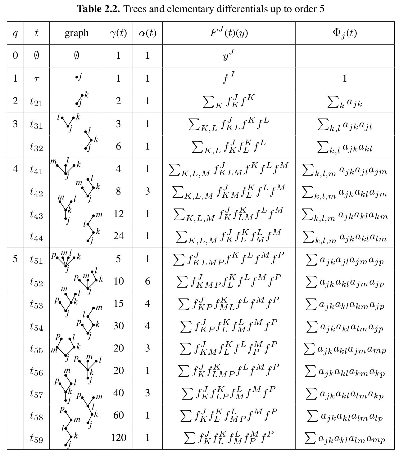
Theorem (from Hairer, Nørsett, and Wanner)

A Runge-Kutta method is of order \(p\) if and only if

\[ \gamma(\mathcal t) \sum_{j} b_j \Phi_j(t) = 1 \]

for all trees \(t\) of order \(\le p\).

For a linear autonomous equation

\[ \dot u = A u \]

we only need one additional order condition per order of accuracy because \(f'' = 0\). These conditions can also be derived by equating derivatives of the stability function \(R(z)\) with the exponential \(e^z\). For a linear non-autonomous equation

\[ \dot u = A(t) u + g(t) \]

or more generally, an autonomous system with quadratic right hand side,

\[ \dot u = B (u \otimes u) + A u + C \]

where \(B\) is a rank 3 tensor, we have \(f''' = 0\), thus limiting the number of order conditions.

previous

2021-09-29 Handling stiffness

next

2021-10-04 RK methods for stiff problems