.ipynb .pdf

repository open issue

Binder Live Code

Contents

2021-10-08 Finite Difference in 2D

Last time

• Accuracy vs cost tradeoffs for ODE integrators

• Stiff and non-stiff problems, discussion of costs

Today

• FD methods in 2D

• Cost profile

• The need for fast algebraic solvers

using Plots
using LinearAlgebra
using SparseArrays
using Zygote

default(linewidth=4)

function newton(residual, jacobian, u0; maxits=20)
    u = u0
    uhist = [copy(u)]
    normhist = []
    for k in 1:maxits
        f = residual(u)
        push!(normhist, norm(f))
        J = jacobian(u)
        delta_u = - J \ f
        u += delta_u
        push!(uhist, copy(u))
    end
    uhist, normhist
end

function plot_stability(Rz, title; xlims=(-2, 2), ylims=(-2, 2))
    x = LinRange(xlims[1], xlims[2], 100)
    y = LinRange(ylims[1], ylims[2], 100)
    heatmap(x, y, (x, y) -> abs(Rz(x + 1im*y)), c=:bwr, clims=(0, 2), aspect_ratio=:equal, title=title)
end

plot_stability (generic function with 1 method)

Extending advection-diffusion to 2D

1 dimension

(19)\[\begin{align} u_t + (- \kappa u_x + w u)_x &= f(x) & \text{ on } \Omega &= (a,b) \\ u(a) &= g_D(a) & u'(b) &= g_N(b) \end{align}\]

• Cell Peclet number \(\mathrm{Pe}_h = \frac{\lvert w \rvert h}{\kappa}\)

  • \(\mathrm{Pe}_h \lesssim 1\) avoids oscillations

  • \(\mathrm{Pe}_h \gtrsim 1\) is non-stiff for time-dependent model

• Centered versus upwind for advection

• Need uniformly bounded \(\kappa \ge \epsilon > 0\)

• “Strong form” not defined at discontinuities in \(\kappa\)

  • Works okay using divergence form and fluxes at staggered points

2 dimensions

(20)\[\begin{align} u_t + \nabla\cdot\big(- \kappa \nabla u + \mathbf{w} u \big) &= f(x,y) & \text{ on } \Omega & \subset \mathbb R^2 \\ u|_{\Gamma_D} &= g_D(x,y) \\ (-\kappa \nabla u + \mathbf w u) \cdot \hat n|_{\Gamma_N} &= g_N(x,y) \end{align}\]

• \(\Omega\) is some well-connected open set (we will assume simply connected) and the Dirichlet boundary \(\Gamma_D \subset \partial \Omega\) is nonempty.

• Finite difference methods don’t have an elegant/flexible way to specify boundaries

• We’ll choose \(\Omega = (-1, 1) \times (-1, 1)\)

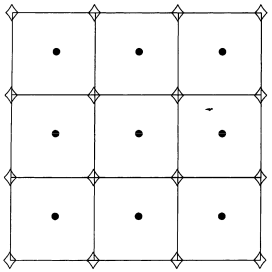
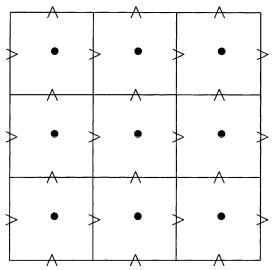
On finite difference grids

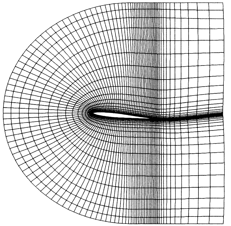
• Non-uniform grids can mesh “special” domains

  • Rare in 3D; overset grids, immersed boundary methods

• Concept of staggering is complicated/ambiguous

Time-independent advection-diffusion

Advection

\[ \nabla\cdot(\mathbf w u) = \mathbf w \cdot \nabla u + (\nabla\cdot \mathbf w) u\]

If we choose divergence-free \(\mathbf w\), we can use the stencil

\[\begin{split} \mathbf w \cdot \nabla u \approx \frac 1 h \begin{bmatrix} & w_2 & \\ -w_1 & & w_1 \\ & -w_2 & \end{bmatrix} \!:\! \begin{bmatrix} u_{i-1, j+1} & u_{i, j+1} & u_{i+1,j+1} \\ u_{i-1, j} & u_{i, j} & u_{i+1,j} \\ u_{i-1, j-1} & u_{i, j-1} & u_{i+1,j-1} \\ \end{bmatrix} \end{split}\]

Diffusion

\[ -\nabla\cdot(\kappa \nabla u) = -\kappa \nabla\cdot \nabla u - \nabla\kappa\cdot \nabla u\]

• When would you trust this decomposition?

• If we have constant \(\kappa\), we can write

  \[\begin{split} -\kappa \nabla\cdot \nabla u \approx \frac{\kappa}{h^2} \begin{bmatrix} & -1 & \\ -1 & 4 & -1 \\ & -1 & \end{bmatrix} \!:\! \begin{bmatrix} u_{i-1, j+1} & u_{i, j+1} & u_{i+1,j+1} \\ u_{i-1, j} & u_{i, j} & u_{i+1,j} \\ u_{i-1, j-1} & u_{i, j-1} & u_{i+1,j-1} \\ \end{bmatrix} \end{split}\]

Advection-diffusion in code

function advdiff_matrix(n; kappa=1, wind=[1, 1]/sqrt(2))
    h = 2 / n
    rows = Vector{Int64}()
    cols = Vector{Int64}()
    vals = Vector{Float64}()
    idx(i, j) = (i-1)*n + j
    stencil_advect = [-wind[1], -wind[2], 0, wind[1], wind[2]] / h
    stencil_diffuse = [-1, -1, 4, -1, -1] * kappa / h^2
    for i in 1:n
        for j in 1:n
            if i in [1, n] || j in [1, n]
                push!(rows, idx(i, j))
                push!(cols, idx(i, j))
                push!(vals, 1.)
            else
                append!(rows, repeat([idx(i,j)], 5))
                append!(cols, [idx(i-1,j), idx(i,j-1), idx(i,j), idx(i+1,j), idx(i,j+1)])
                append!(vals, stencil_advect + stencil_diffuse)
            end
        end
    end
    sparse(rows, cols, vals)
end

advdiff_matrix (generic function with 1 method)

Spy the matrix

A = advdiff_matrix(10, wind=[1, 3], kappa=.1)
clim = norm(vec(A), Inf)
spy(A, marker=(:square, 3), c=:bwr, clims=(-clim, clim))

A = advdiff_matrix(20, wind=[0, 0], kappa=.1)
ev = eigvals(Matrix(A))
scatter(real(ev), imag(ev))

Plot a solution

n = 100
x = LinRange(-1, 1, n)
y = x
f = cos.(pi*x/2) * cos.(pi*y/2)'
heatmap(x, y, f, aspect_ratio=:equal)

A = advdiff_matrix(n, wind=[3,1], kappa=.01)
u = A \ vec(f)
heatmap(x, y, reshape(u, n, n), aspect_ratio=:equal)

• What happens when advection dominates?

• As you refine the grid?

Cost breadown and optimization

using ProfileSVG
function assemble_and_solve(n)
    A = advdiff_matrix(n)
    x = LinRange(-1, 1, n)
    f = cos.(pi*x/2) * cos.(pi*x/2)'
    u = A \ vec(f)
end

@profview assemble_and_solve(600)

What’s left?

• Symmetric Dirichlet boundary conditions

• Symmetric Neumann boundary conditions

• Verification with method of manufactured solutions

• Non-uniform grids

• Upwinding for advection-dominated problems

• Variable coefficients

• Time-dependent problems

• Fast algebraic solvers

previous

2021-10-04 RK methods for stiff problems

next

2021-10-13 Wave equations