
2022-11-09 Solid Mechanics
Contents
2022-11-09 Solid Mechanics#
Last time#
Stabilized methods for transport
VMS and SUPG
FE interfaces
Today#
Mixed finite elements
Intro to solid mechanics, Ratel
using Plots
default(linewidth=3)
using LinearAlgebra
using SparseArrays
using FastGaussQuadrature
import NLsolve: nlsolve

function my_spy(A)
    cmax = norm(vec(A), Inf)
    s = max(1, ceil(120 / size(A, 1)))
    spy(A, marker=(:square, s), c=:diverging_rainbow_bgymr_45_85_c67_n256, clims=(-cmax, cmax))
end

function vander_legendre_deriv(x, k=nothing)
    if isnothing(k)
        k = length(x) # Square by default
    end
    m = length(x)
    Q = ones(m, k)
    dQ = zeros(m, k)
    Q[:, 2] = x
    dQ[:, 2] .= 1
    for n in 1:k-2
        Q[:, n+2] = ((2*n + 1) * x .* Q[:, n+1] - n * Q[:, n]) / (n + 1)
        dQ[:, n+2] = (2*n + 1) * Q[:,n+1] + dQ[:,n]
    end
    Q, dQ
end

function febasis(P, Q, quadrature=gausslegendre)
    x, _ = gausslobatto(P)
    q, w = quadrature(Q)
    Pk, _ = vander_legendre_deriv(x)
    Bp, Dp = vander_legendre_deriv(q, P)
    B = Bp / Pk
    D = Dp / Pk
    x, q, w, B, D
end

function fe1_mesh(P, nelem)
    x = LinRange(-1, 1, nelem+1)
    rows = Int[]
    cols = Int[]
    for i in 1:nelem
        append!(rows, (i-1)*P+1:i*P)
        append!(cols, (i-1)*(P-1)+1:i*(P-1)+1)
    end
    x, sparse(cols, rows, ones(nelem*P))'
end

function xnodal(x, P)
    xn = Float64[]
    xref, _ = gausslobatto(P)
    for i in 1:length(x)-1
        xL, xR = x[i:i+1]
        append!(xn, (xL+xR)/2 .+ (xR-xL)/2 * xref[1+(i>1):end])
    end
    xn
end

struct FESpace
    P::Int
    Q::Int
    nelem::Int
    x::Vector
    xn::Vector
    Et::SparseMatrixCSC{Float64, Int64}
    q::Vector
    w::Vector
    B::Matrix
    D::Matrix
    function FESpace(P, Q, nelem, quadrature=gausslegendre)
        x, E = fe1_mesh(P, nelem)
        xn = xnodal(x, P)
        _, q, w, B, D = febasis(P, Q, quadrature)
        new(P, Q, nelem, x, xn, E', q, w, B, D)
    end
end

# Extract out what we need for element e
function fe_element(fe, e)
    xL, xR = fe.x[e:e+1]
    q = (xL+xR)/2 .+ (xR-xL)/2*fe.q
    w = (xR - xL)/2 * fe.w
    E = fe.Et[:, (e-1)*fe.P+1:e*fe.P]'
    dXdx = ones(fe.Q) * 2 / (xR - xL)
    q, w, E, dXdx
end

function fe_residual(u_in, fe, fq; bci=[1], bcv=[1.])
    u = copy(u_in); v = zero(u)
    u[bci] = bcv
    for e in 1:fe.nelem
        q, w, E, dXdx = fe_element(fe, e)
        B, D = fe.B, fe.D
        ue = E * u
        uq = B * ue
        Duq = dXdx .* (D * ue)
        f0, f1 = fq(q, uq, Duq)
        ve = B' * (w .* f0) + D' * (dXdx .* w .* f1)
        v += E' * ve
    end
    v[bci] = u_in[bci] - u[bci]
    #println("residual")
    v
end

function fe_jacobian(u_in, fe, dfq; bci=[1], bcv=[1.])
    u = copy(u_in); u[bci] = bcv
    rows, cols, vals = Int[], Int[], Float64[]
    for e in 1:fe.nelem
        q, w, E, dXdx = fe_element(fe, e)
        B, D, P = fe.B, fe.D, fe.P
        ue = E * u
        uq = B * ue; Duq = dXdx .* (D * ue)
        K = zeros(P, P)
        for j in 1:fe.P
            du = B[:,j]
            Ddu = dXdx .* D[:,j]
            df0, df1 = dfq(q, uq, du, Duq, Ddu)
            K[:,j] = B' * (w .* df0) + D' * (dXdx .* w .* df1)
        end
        inds = rowvals(E')
        append!(rows, kron(ones(P), inds))
        append!(cols, kron(inds, ones(P)))
        append!(vals, vec(K))
    end
    A = sparse(rows, cols, vals)
    A[bci, :] .= 0; A[:, bci] .= 0
    A[bci,bci] = diagm(ones(length(bci)))
    A
end
fe_jacobian (generic function with 1 method)
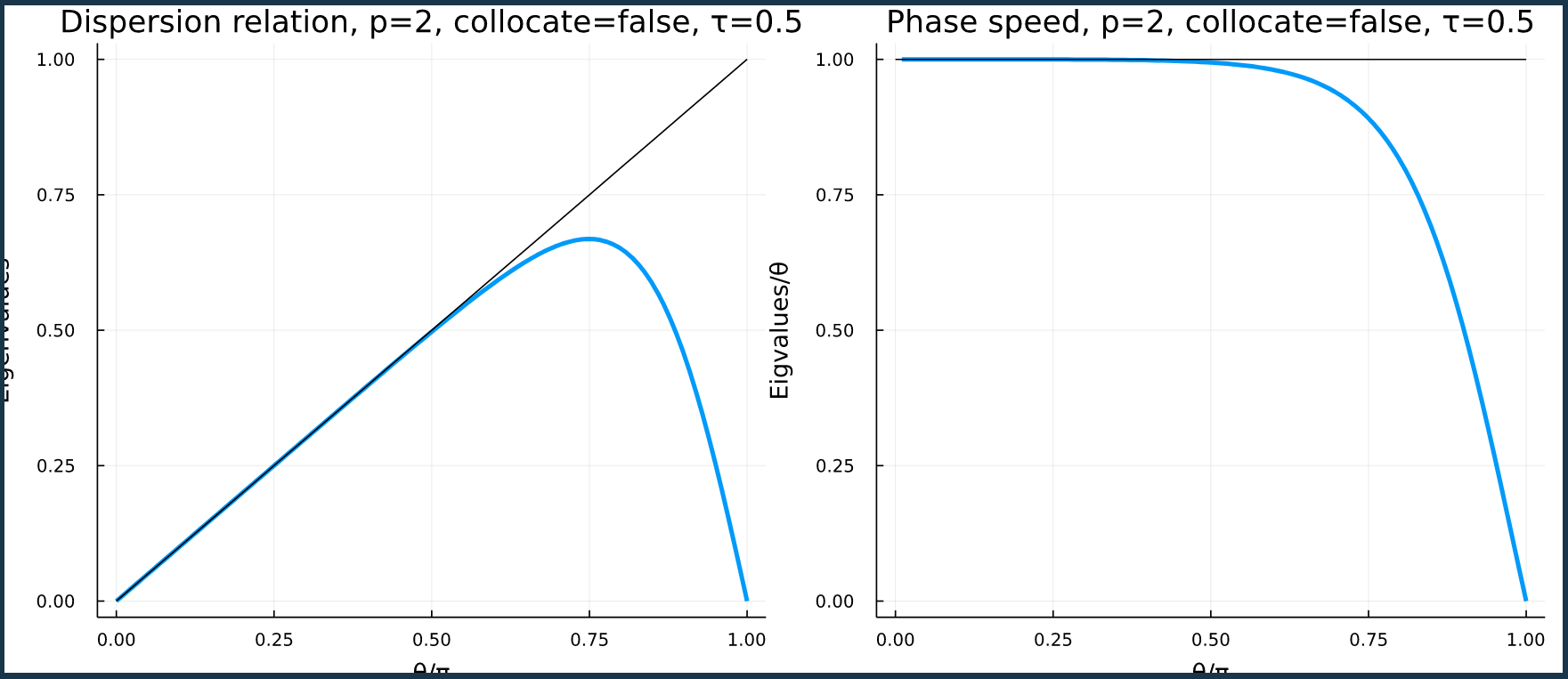
SUPG dispersion diagram (consistent)#
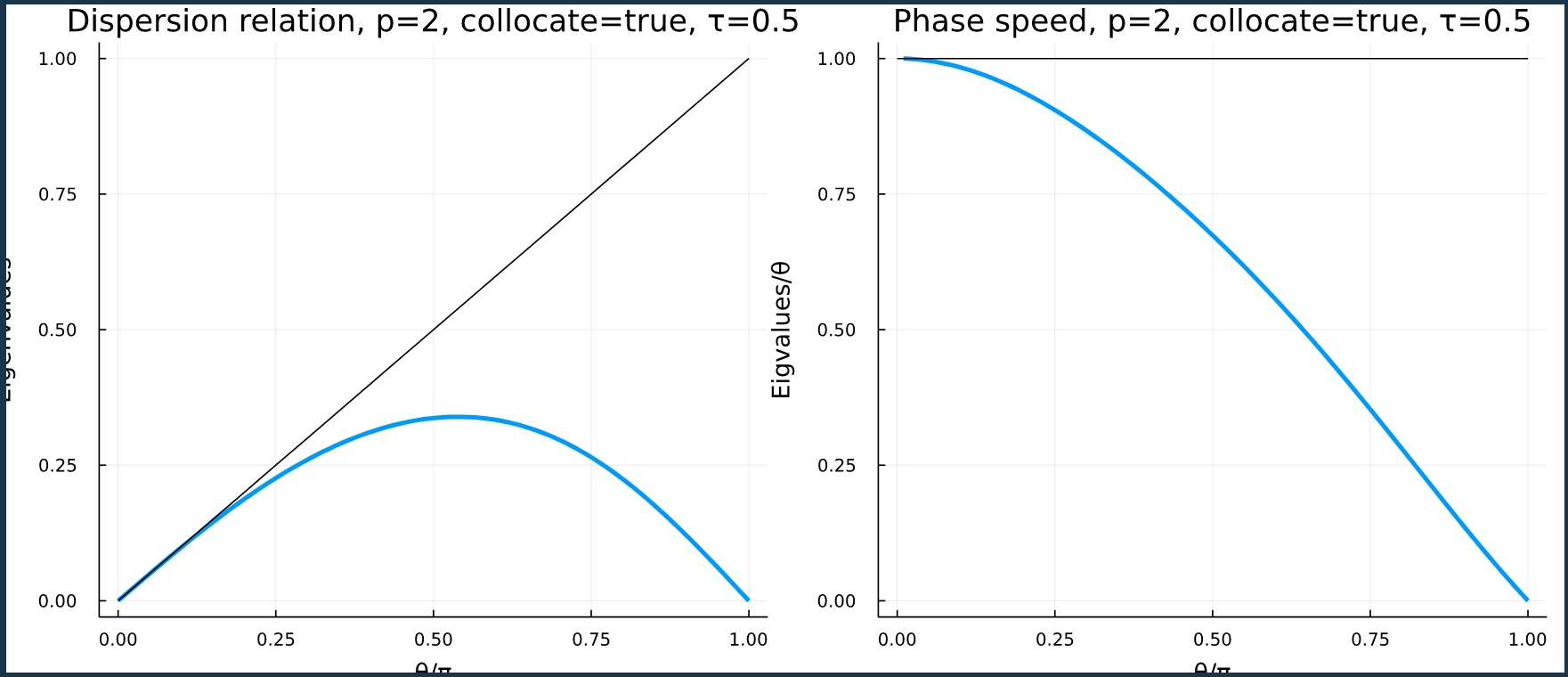
SUPG dispersion diagram (lumped)#
Finite element interfaces: Deal.II#
Deal.II step-7
for e in elems:
    fe_values.reinit()
    for q in q_points:
        for i in test_functions:
            for j in trial_functions
                K_e[i,j] += ...
            f_e[i] += ...
    for f in e.faces:
        if f.at_boundary():
            fe_face_values.reinit()
            for q in q_points:
                ...
Finite element interfaces: MOOSE#
Materials#
Can be written without knowledge of finite elements
Registration allows libraries of materials (some in MOOSE, others packaged separatle)
Example: crystal plasticity
Code is C++, so can do dirty things
table lookups, proprietary code
implicit materials (Newton solve at each quadrature point)
Composition in configuration files#
Add fields and coupling
Select materials from libraries
Multiphysics composition
Multiscale coupling
Graphical interface: Peacock#
Periodic table of finite elements#
Careful choice of mixed elements allows exactly satisfying discrete identities#
Generalized concept: Finite Element Exterior Calculus (FEEC)
Improved stability or numerical properties
Higher order of accuracy for quantity of interest despite non-smooth problem
\(H^1\) Poisson#
Find \(p\) such that
Mixed Poisson#
Find \(\mathbf u, p\) such that
Dirichlet (essential) and Neumann (natural) boundary conditions are swapped, and we get a “saddle point” linear problem $$\begin{pmatrix} M & B^T \ B & 0 \end{pmatrix} \begin{pmatrix} \mathbf u \ p \end{pmatrix} =
$\( With appropriate choice of spaces, \)p,q\( can live in a piecewise constant space while attaining second order accuracy in the fluxes \)\mathbf u$.
Problems with constraints#
Stokes: (slow) incompressible flow#
Find velocity \(\mathbf u\) and pressure \(p\) such that
where \(\nabla^s \mathbf u\) is the symmetric part of the \(3\times 3\) gradient \(\nabla \mathbf u\).
Weak form: find \((\mathbf u, p)\) such that
Inf-sup stability#
For this problem to be well posed, it is necessary that the divergence of velocity spans the pressure space “nicely”. This is quantified by the “inf-sup constant” (aka. Ladyzhenskaya–Babuška–Brezzi constant)
The method loses accuracy if \(\beta\) decays: you want it to stay of order 1 uniformly. Stability can be quantified numerically by solving an eigenvalue problem (1993). This short paper has many figures quantifying stable and unstable elements.
Solid mechanics: Ratel Theory Guide#
Material coordinates#
The current configuration \(x\) is a function of the initial configuration \(X\). We typically solve for displacement \(u = x - X\), and define the deformation gradient
Conservation#
Mass by definition of density#
Momentum by equations we solve#
Angular momentum by symmetry of stress and strain tensors#
Momentum balance in initial configuration#
where \(\mathbf F = I + H\) and \(\mathbf S\) is the symmetric stress tensor (Second Piola-Kirchhoff tensor).
Strain measures#
Stress \(\mathbf S\) must be defined as a function of displacement. A common choice is to define the right Cauchy-Green tensor
This has value \(I\) for zero strain. A better formulation uses
Neo-Hookean model#
Strain energy density \begin{aligned} \psi \left(\mathbf{E} \right) &= \frac{\lambda}{2} \left( \log J \right)^2 - \mu \log J + \frac \mu 2 \left( \operatorname{trace} \mathbf{C} - 3 \right) \ &= \frac{\lambda}{2} \left( \log J \right)^2 - \mu \log J + \mu \operatorname{trace} \mathbf{E}, \end{aligned}
Stable evaluation#

Paper on Efficient Methods#
