
2021-12-01 Finite Volume methods
Last time
Notes on unstructured meshing workflow
Finite volume methods for hyperbolic conservation laws
Riemann solvers for scalar equations
Shocks and the Rankine-Hugoniot condition
Rarefactions and entropy solutions
Today
Higher order methods
Godunov’s Theorem
Slope reconstruction
Slope limiting
using LinearAlgebra
using Plots
default(linewidth=4)

struct RKTable
    A::Matrix
    b::Vector
    c::Vector
    function RKTable(A, b)
        s = length(b)
        A = reshape(A, s, s)
        c = vec(sum(A, dims=2))
        new(A, b, c)
    end
end

rk4 = RKTable([0 0 0 0; .5 0 0 0; 0 .5 0 0; 0 0 1 0], [1, 2, 2, 1] / 6)

function ode_rk_explicit(f, u0; tfinal=1., h=0.1, table=rk4)
    u = copy(u0)
    t = 0.
    n, s = length(u), length(table.c)
    fY = zeros(n, s)
    thist = [t]
    uhist = [u0]
    while t < tfinal
        tnext = min(t+h, tfinal)
        h = tnext - t
        for i in 1:s
            ti = t + h * table.c[i]
            Yi = u + h * sum(fY[:,1:i-1] * table.A[i,1:i-1], dims=2)
            fY[:,i] = f(ti, Yi)
        end
        u += h * fY * table.b
        t = tnext
        push!(thist, t)
        push!(uhist, u)
    end
    thist, hcat(uhist...)
end

function testfunc(x)
    max(1 - 4*abs.(x+2/3),
        abs.(x) .< .2,
        (2*abs.(x-2/3) .< .5) * cospi(2*(x-2/3)).^2
    )
end

riemann_advection(uL, uR) = 1*uL # velocity is +1

function fv_solve1(riemann, u_init, n, tfinal=1)
    h = 2 / n
    x = LinRange(-1+h/2, 1-h/2, n) # cell midpoints (centroids)
    idxL = 1 .+ (n-1:2*n-2) .% n
    idxR = 1 .+ (n+1:2*n) .% n
    function rhs(t, u)
        fluxL = riemann(u[idxL], u)
        fluxR = riemann(u, u[idxR])
        (fluxL - fluxR) / h
    end
    thist, uhist = ode_rk_explicit(
        rhs, u_init.(x), h=h, tfinal=tfinal)
    x, thist, uhist
end

function riemann_burgers(uL, uR)
    flux = zero(uL)
    for i in 1:length(flux)
        fL = flux_burgers(uL[i])
        fR = flux_burgers(uR[i])
        flux[i] = if uL[i] > uR[i] # shock
            max(fL, fR)
        elseif uL[i] > 0 # rarefaction all to the right
            fL
        elseif uR[i] < 0 # rarefaction all to the left
            fR
        else
            0
        end
    end
    flux
end

function riemann_traffic(uL, uR)
    flux = zero(uL)
    for i in 1:length(flux)
        fL = flux_traffic(uL[i])
        fR = flux_traffic(uR[i])
        flux[i] = if uL[i] < uR[i] # shock
            min(fL, fR)
        elseif uL[i] < .5 # rarefaction all to the right
            fL
        elseif uR[i] > .5 # rarefaction all to the left
            fR
        else
            flux_traffic(.5)
        end
    end
    flux
end
riemann_traffic (generic function with 1 method)
Godunov’s Theorem (1954)
Linear numerical methods
For our purposes, monotonicity is equivalent to positivity preservation,
Discontinuities
A numerical method for representing a discontinuous function on a stationary grid can be no better than first order accurate in the \(L^1\) norm,
In light of these two observations, we may still ask for numerical methods that are more than first order accurate for smooth solutions, but those methods must be nonlinear.
Slope Reconstruction
One method for constructing higher order methods is to use the state in neighboring elements to perform a conservative reconstruction of a piecewise polynomial, then compute numerical fluxes by solving Riemann problems at the interfaces. If \(x_i\) is the center of cell \(i\) and \(g_i\) is the reconstructed gradient inside cell \(i\), our reconstructed solution is
Slope limiting
We will determine gradients by “limiting” the above slope using a nonlinear function that reduces to 1 when the solution is smooth. There are many ways to express limiters and our discussion here roughly follows Berger, Aftosmis, and Murman (2005).
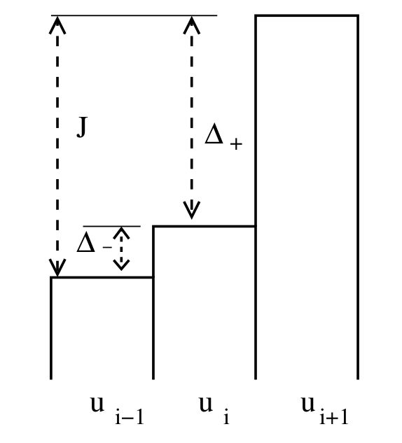
We will express a slope limiter in terms of the ratio
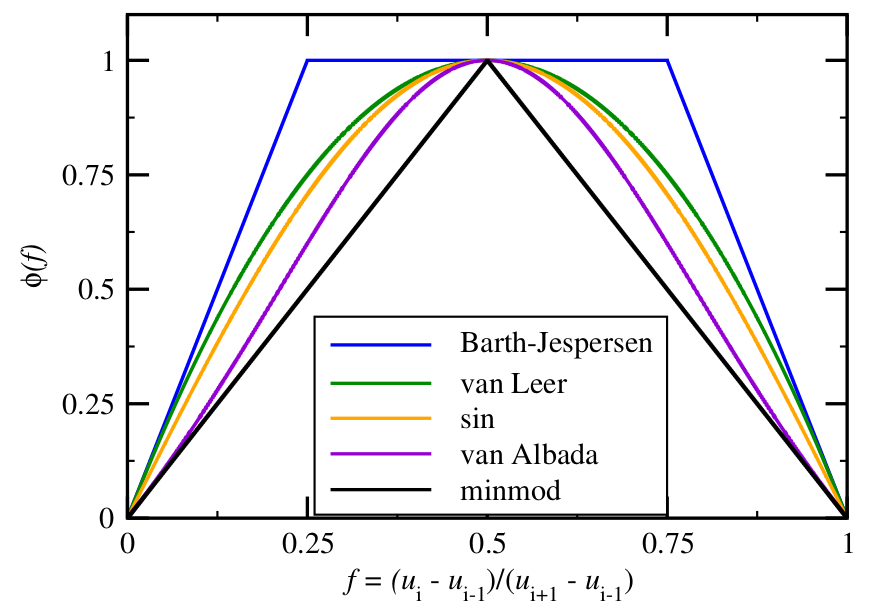 All of these limiters are second order accurate and TVD; those that fall below minmod are not second order accurate and those that are above Barth-Jesperson are not second order accurate, not TVD, or produce artifacts.
Common limiters
limit_zero(r) = 0
limit_none(r) = 1
limit_minmod(r) = max(min(2*r, 2*(1-r)), 0)
limit_sin(r) = (0 < r && r < 1) * sinpi(r)
limit_vl(r) = max(4*r*(1-r), 0)
limit_bj(r) = max(0, min(1, 4*r, 4*(1-r)))
limiters = [limit_zero limit_none limit_minmod limit_sin limit_vl limit_bj];
plot(limiters, label=limiters, xlims=(-.1, 1.1))

A slope-limited solver
function fv_solve2(riemann, u_init, n, tfinal=1, limit=limit_sin)
    h = 2 / n
    x = LinRange(-1+h/2, 1-h/2, n) # cell midpoints (centroids)
    idxL = 1 .+ (n-1:2*n-2) .% n
    idxR = 1 .+ (n+1:2*n) .% n
    function rhs(t, u)
        jump = u[idxR] - u[idxL]
        r = (u - u[idxL]) ./ jump
        r[isnan.(r)] .= 0
        g = limit.(r) .* jump / 2h
        fluxL = riemann(u[idxL] + g[idxL]*h/2, u - g*h/2)
        fluxR = fluxL[idxR]
        (fluxL - fluxR) / h
    end
    thist, uhist = ode_rk_explicit(
        rhs, u_init.(x), h=h, tfinal=tfinal)
    x, thist, uhist
end
fv_solve2 (generic function with 3 methods)
x, thist, uhist = fv_solve2(riemann_advection, testfunc, 100, .5,
    limit_sin)
plot(x, uhist[:,1:10:end], legend=:none)
