2023-11-29 CEED Fluids#
Last time#
Equations
Conservation
Choice of variables
Today#
SUPG stabilization
Solvers
Boundary conditions
using Plots
default(linewidth=3)
using LinearAlgebra
using SparseArrays
Conservation of mass, momentum, and energy#
Equation of state
\begin{aligned} \bm{F}(\bm{q}) &= \underbrace{\begin{pmatrix} \rho\bm{u}\ {\rho \bm{u} \otimes \bm{u}} + P \bm{I}3 \ {(E + P)\bm{u}} \end{pmatrix}}{\bm F_{\text{adv}}} + \underbrace{\begin{pmatrix} 0 \
\bm{\sigma} \
\bm{u} \cdot \bm{\sigma} - k \nabla T \end{pmatrix}}{\bm F{\text{diff}}},\ S(\bm{q}) &=
- (62)#\[\begin{pmatrix} 0\\ \rho g \bm{\hat{k}}\\ 0 \end{pmatrix}\]
\end{aligned}
Choice of variables#
Acoustic wave speed#
material |
speed |
|---|---|
air |
340 m/s |
water |
1500 m/s |
Mach number#
Primitive variables#
Using the equation of state, we can write \(\bm y(\bm q)\) or \(\bm q(\bm y)\). But these transformations are ill conditioned for \(\mathrm{Ma} \ll 1\).
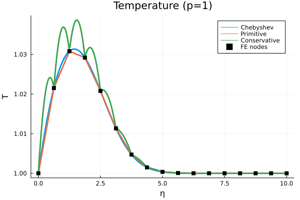
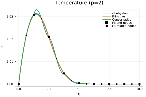
Blasius profile (thanks, Leila Ghaffari)#
Take an analytic Blasius profile.
Primitive: Write \(\bm y\) in a piecewise linear space with nodally exact values.Conservative: Write \(\bm q\) in a piecewise linear space with nodally exact values.
Stabilization#
Boundary term needs to be replaced with actual boundary conditions
The strong form term \(\nabla\cdot \bm F(\bm y)\)
is ill-defined at shocks or discontinuous materials
involves the second derivative of velocity and temperature; many ignore for linear elements, but it’s better to use a (lumped) projection.
Time integration#
Fully implicit \(G(t, \bm y, \dot{\bm y}) = 0\) with generalized alpha.
Newton method, usually about 3 iterations per time step.
Krylov method
GMRES when using a strong preconditioner
Block Jacobi/incomplete LU
BCGS(\(\ell\)) with a weak preconditioner
Point-block Jacobi
Boundary conditions (ref: Mengaldo et al (2014))#
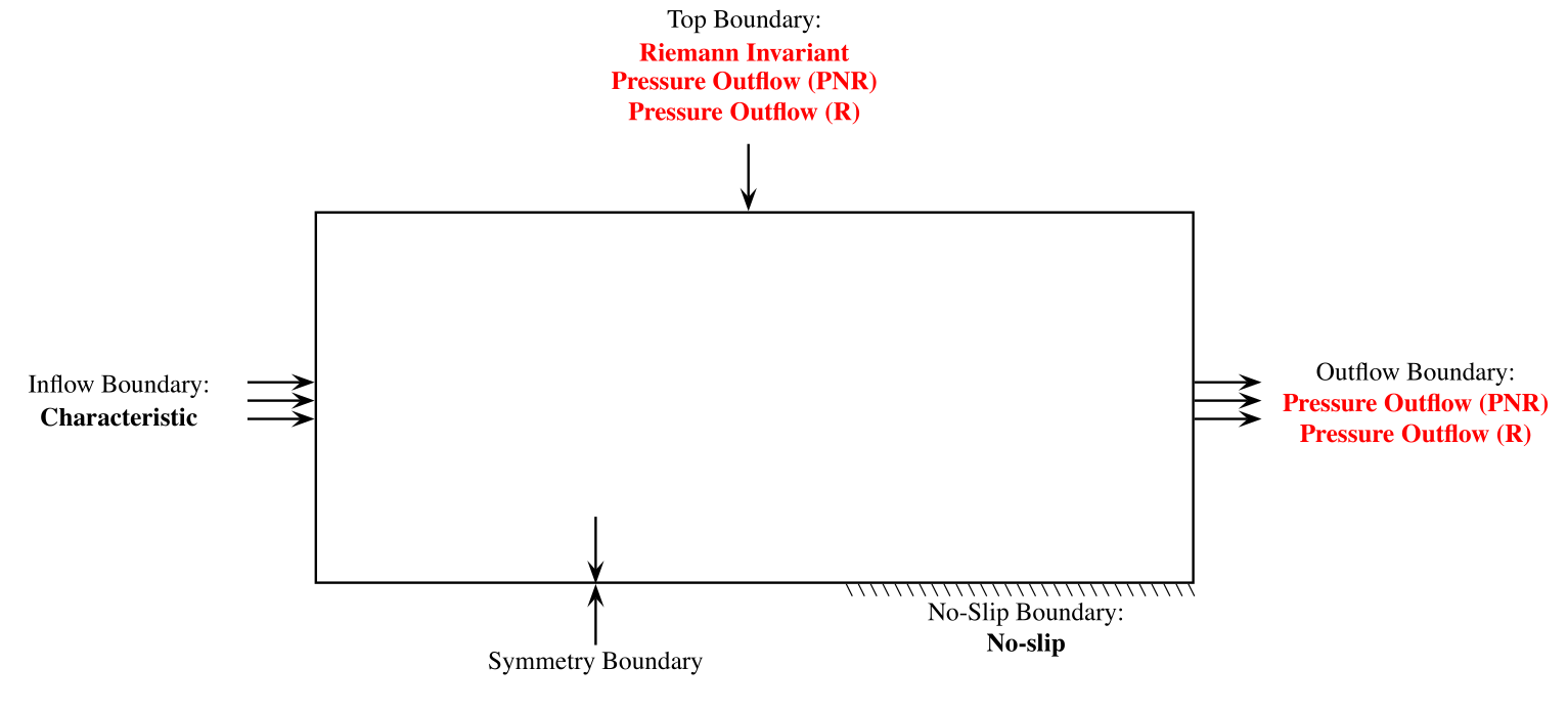
Boundary conditions#
Unlike solid mechanics, the “natural” boundary condition is not physical (it’s like a free surface). So we need boundary conditions all around.
Symmetry (free slip)#
Normal velocity = 0, no boundary integral
Wall (no-slip)#
Total velocity = 0
Can prescribe temperature (heat sink) or leave it insulated (more complicated for conservative variables)
Freestream boundaries#
Unified way to handle inflow and outflow (sometimes both).
Requires solving a “Riemann problem”
Viscous inflow#
Prescribe velocity and temperature, compute boundary integral for energy flux.
Viscous outflow#
Prescribe pressure, compute flux with modified ghost pressure \(2 P_{\text{ext}} - P_{\text{int}}\)
Compute viscous flux based on interior values
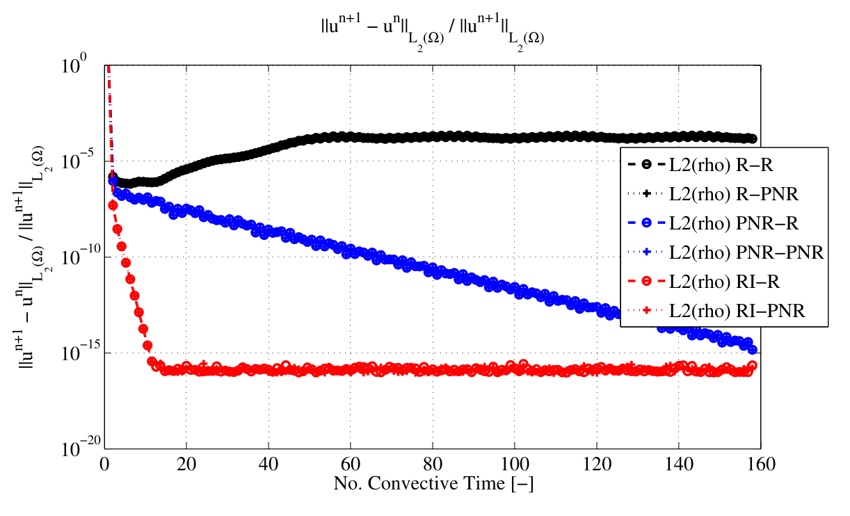
Convergence to steady state (from Mengaldo)#
Freestream wave test problem#
$ mpiexec -n 6 build/fluids-navierstokes -options_file examples/fluids/newtonianwave.yaml
HLL#
HLLC#
Open Problem:#
Turbulent viscous inflow and outflow with non-reflecting boundary conditions.#
Boundary layers for turbulent flow#
dymin = 2.66077e-5
alpha_BL = 1.05
dymax_BL = 0.00266077
alpha_OBL = 1.2
dymax_OBL = 0.1
delta = 0.21

function phasta_spacing(n)
    y = zeros(n+1)
    h = zeros(n+1)
    h[1] = dymin
    for i in 2:n+1
        y[i] = y[i-1] + h[i-1]
        h[i] = if y[i] < delta
            min(h[i-1] * alpha_BL, dymax_BL)
        else
            min(h[i-1] * alpha_OBL, dymax_OBL)
        end
    end
    y, h
end

h_IBL(s) = dymin * alpha_BL ^ (s*n)
H_IBL(s) = dymin * alpha_BL ^ (s*n) / log(alpha_BL)

function fractional_spacing(x)
    # find first junction
    x_IBL = log(dymax_BL / dymin) / (n * log(alpha_BL))

    # find second junction by integrating
    y_IBL = H_IBL(x_IBL) - H_IBL(0)
    # find x such that y_IBL + dymax_BL * (x - x_IBL)*n = delta
    x_delta = x_IBL + (delta - y_IBL) / (dymax_BL * n)

    # find third junction
    x_OBL = x_delta + log(dymax_OBL / dymax_BL) / (n * log(alpha_OBL))

    if x < x_IBL
        h_IBL(x)
    elseif x < x_delta
        dymax_BL
    elseif x < x_OBL
        dymax_BL * alpha_OBL ^ ((x - x_delta)*n)
    else
        dymax_OBL
    end
end
fractional_spacing (generic function with 1 method)
n = 200
y, h = phasta_spacing(n)
plot((0:n)/n, h, yscale=:log10, legend=:none, ylabel="\$h\$", xlabel="fractional elements from wall")
plot!(fractional_spacing)
Geometric spacing near the wall
Aspect ratio \(10\) to \(10^5\)
Wall-resolved or wall-modeled
Turbulent boundary layer
Far field
In unstructured CFD, most elements are close to a wall.
Running on Alpine#
$ ssh login.rc.colorado.edu
rc$ module load slurm/alpine
rc$ acompile
acompile$ . /projects/jeka2967/activate.bash
$ git clone \
    https://github.com/CEED/libCEED
$ cd libCEED
$ make build/fluids-navierstokes
$ mpiexec -n 1 build/fluids-navierstokes \
    -options_file \
    examples/fluids/gaussianwave.yaml
Running in Docker#
Clone the libCEED repository and cd libCEED
host$ docker run -it --rm -v $(pwd):/work registry.gitlab.com/micromorph/ratel
$ make build/fluids-navierstokes
$ mpiexec -n 2 build/fluids-navierstokes -options_file FILE.yaml
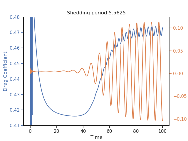
Vortex shedding#
Problem setup#
examples/fluids/vortexshedding.yamlMach 0.01
Reynolds 100