2023-12-06 Systems

2023-12-06 Systems#

Last time#

Godunov’s Theorem
Slope reconstruction and limiting

Today#

Hyperbolic systems
Rankine-Hugoniot and Riemann Invariants
Exact Riemann solvers
Approximate Riemann solvers
Multi-dimensional generalizations

using LinearAlgebra
using Plots
default(linewidth=3)

struct RKTable
    A::Matrix
    b::Vector
    c::Vector
    function RKTable(A, b)
        s = length(b)
        A = reshape(A, s, s)
        c = vec(sum(A, dims=2))
        new(A, b, c)
    end
end

rk4 = RKTable([0 0 0 0; .5 0 0 0; 0 .5 0 0; 0 0 1 0], [1, 2, 2, 1] / 6)

function ode_rk_explicit(f, u0; tfinal=1., h=0.1, table=rk4)
    u = copy(u0)
    t = 0.
    n, s = length(u), length(table.c)
    fY = zeros(n, s)
    thist = [t]
    uhist = [u0]
    while t < tfinal
        tnext = min(t+h, tfinal)
        h = tnext - t
        for i in 1:s
            ti = t + h * table.c[i]
            Yi = u + h * sum(fY[:,1:i-1] * table.A[i,1:i-1], dims=2)
            fY[:,i] = f(ti, Yi)
        end
        u += h * fY * table.b
        t = tnext
        push!(thist, t)
        push!(uhist, u)
    end
    thist, hcat(uhist...)
end

function testfunc(x)
    max(1 - 4*abs.(x+2/3),
        abs.(x) .< .2,
        (2*abs.(x-2/3) .< .5) * cospi(2*(x-2/3)).^2
    )
end

flux_advection(u) = u
flux_burgers(u) = u^2/2
flux_traffic(u) = u * (1 - u)

riemann_advection(uL, uR) = 1*uL # velocity is +1

function fv_solve1(riemann, u_init, n, tfinal=1)
    h = 2 / n
    x = LinRange(-1+h/2, 1-h/2, n) # cell midpoints (centroids)
    idxL = 1 .+ (n-1:2*n-2) .% n
    idxR = 1 .+ (n+1:2*n) .% n
    function rhs(t, u)
        fluxL = riemann(u[idxL], u)
        fluxR = riemann(u, u[idxR])
        (fluxL - fluxR) / h
    end
    thist, uhist = ode_rk_explicit(rhs, u_init.(x), h=h, tfinal=tfinal)
    x, thist, uhist
end

function riemann_burgers(uL, uR)
    flux = zero(uL)
    for i in 1:length(flux)
        fL = flux_burgers(uL[i])
        fR = flux_burgers(uR[i])
        flux[i] = if uL[i] > uR[i] # shock
            max(fL, fR)
        elseif uL[i] > 0 # rarefaction all to the right
            fL
        elseif uR[i] < 0 # rarefaction all to the left
            fR
        else
            0
        end
    end
    flux
end

function riemann_traffic(uL, uR)
    flux = zero(uL)
    for i in 1:length(flux)
        fL = flux_traffic(uL[i])
        fR = flux_traffic(uR[i])
        flux[i] = if uL[i] < uR[i] # shock
            min(fL, fR)
        elseif uL[i] < .5 # rarefaction all to the right
            fL
        elseif uR[i] > .5 # rarefaction all to the left
            fR
        else
            flux_traffic(.5)
        end
    end
    flux 
end

limit_zero(r) = 0
limit_none(r) = 1
limit_minmod(r) = max(min(2*r, 2*(1-r)), 0)
limit_sin(r) = (0 < r && r < 1) * sinpi(r)
limit_vl(r) = max(4*r*(1-r), 0)
limit_bj(r) = max(0, min(1, 4*r, 4*(1-r)))
limiters = [limit_zero limit_none limit_minmod limit_sin limit_vl limit_bj];

Hyperbolic systems#

\[ U_t + f(U)_x = 0 \]

Isentropic gas dynamics#

(67)#\[\begin{align} U &= \begin{bmatrix} \rho \\ \rho u \end{bmatrix} & f(U) &= \begin{bmatrix} \rho u \\ \rho u^2 + p \end{bmatrix} \end{align}\]

Variable	meaning
\(\rho\)	density
\(u\)	velocity
\(\rho u\)	momentum
\(p\)	pressure

Equation of state \(p(\rho) = C \rho^\gamma\) with \(\gamma = 1.4\) (typical air).
“isothermal” gas dynamics: \(p(\rho) = c^2 \rho\), wave speed \(c\).
Compute as \( \rho u^2 = \frac{(\rho u)^2}{\rho} .\)

Smooth wave structure#

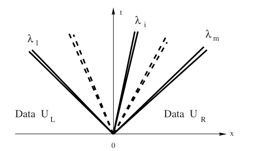
For perturbations of a constant state, systems of equations produce multiple waves with speeds equal to the eigenvalues of the flux Jacobian,

\[\begin{split} f'(U) = \begin{bmatrix} 0 & 1 \\ -u^2 + c^2 & 2 u \end{bmatrix}. \end{split}\]

We can compute the eigenvalues and eigenvectors,

\[ f'(U) = W \Lambda W^{-1} \]

as

(68)#\[\begin{align} W &= \begin{bmatrix} 1 & 1 \\ u-c & u+c \end{bmatrix} & \Lambda &= \begin{bmatrix} u-c & \\ & u+c \end{bmatrix} . \end{align}\]

Riemann problem for systems: shocks#

Given states \(U_L\) and \(U_R\), we will see two waves with some state \(U^*\) in between. There could be two shocks, two rarefactions, or one of each. The type of wave will determine the condition that must be satisfied to connect \(U_L\) to \(U_*\) and \(U_*\) to \(U_R\).

Left-moving wave#

If there is a shock between \(U_L\) and \(U_*\), the Rankine-Hugoniot condition

\[ s \Delta U = \Delta f \]

will be satisfied along with the entropy condition

\[ \lambda_i(U_L) \ge s \ge \lambda_i(U_*) \]

where \(\lambda_i(U)\) is the corresponding eigenvalue of the flux Jacobian \(f'(U)\). The inequality in the entropy condition is strict if the wave is genuinely nonlinear. For isothermal gas dynamics, the Rankine-Hugoniot condition is

(69)#\[\begin{align} (\rho_* - \rho_L) s &= \rho_* u_* - \rho_L u_L \\ (\rho_* u_* - \rho_L u_L) s &= \Big(\rho_* u_*^2 + c^2 \rho_* \Big) - \Big( \rho_L u_L^2 + c^2 \rho_L \Big) \end{align}\]

Solving the first equation for \(s\) and substituting into the second, we compute \begin{split} \frac{(\rho_* u_* - \rho_L u_L)^2}{\rho_* - \rho_L} &= \rho_* u_^2 - \rho_L u_L^2 + c^2 (\rho_ - \rho_L) \ \rho_^2 u_^2 - 2 \rho_* \rho_L u_* u_L + \rho_L^2 u_L^2 &= \rho_* (\rho_* - \rho_L) u_^2 - \rho_L (\rho_ - \rho_L) u_L^2 + c^2 (\rho_* - \rho_L)^2 \ \rho_* \rho_L \Big( u_^2 - 2 u_ u_L + u_L^2 \Big) &= c^2 (\rho_* - \rho_L)^2 \ (u_* - u_L)^2 &= c^2 \frac{(\rho_* - \rho_L)^2}{\rho_* \rho_L} \ u_* - u_L &= \pm c \frac{\rho_* - \rho_L}{\sqrt{\rho_* \rho_L}} \end{split} and will need to use the entropy condition to learn which sign to take.

Admissible shocks#

We need to choose the sign

\[u_* - u_L = \pm c \frac{\rho_* - \rho_L}{\sqrt{\rho_*\rho_L}}\]

The entropy condition requires that

\[ \lambda(U_L) = u_L - c \ge s \ge u_* - c = \lambda(U_*) . \]

Meanwhile, the first Rankine-Hugoniot condition and \(\rho > 0\) provides

\[ \rho_L c \le \rho_L (u_L - s) = \rho_* (u_* - s) \le \rho_* c \]

which is to say that \(\rho_* \ge \rho_L\) and consequently we take the negative sign,

\[ u_* - u_L = - c\frac{\rho_* - \rho_L}{\sqrt{\rho_* \rho_L}} .\]

Right-moving wave#

The same process for the right wave \(\lambda(U) = u + c\) yields a shock when \(\rho_* \ge \rho_R\), in which case the velocity jump is

\[ u_R - u_* = - c \frac{\rho_* - \rho_R}{\sqrt{\rho_* \rho_R}} . \]

Rarefactions#

A rarefaction occurs when

\[ \lambda_i(U_L) < \lambda_i(U_R) \]

Generalized Riemann invariants#

\[ \frac{d U^1}{W_i^1} = \frac{d U^2}{W_i^2} = \dotsb \]

(Derivation of this condition is beyond the scope of this class.)

Isothermal gas dynamics#

\[ \frac{d \rho}{1} = \frac{d (\rho u)}{u - c} \]

across the wave \(\lambda = u-c\). We can rearrange to

\[ (u-c) d \rho = \rho d u + u d \rho \]

or

\[ d u + \frac{c}{\rho} d \rho = 0 . \]

Integration yields

\[ u + \int \frac{c}{\rho} d \rho = u + c \log \rho = \text{constant} . \]

So if we have a rarefaction between \(U_L\) and \(U_*\) then

\[ u_L + c \log \rho_L = u_* + c \log \rho_* . \]

Similarly, for the wave \(\lambda = u + c\), a rarefaction between \(U_*\) and \(U_R\) results in

\[ u_* - c \log \rho_* = u_R - c \log \rho_R . \]

If the rarefaction is sonic, we have \(u_0 - c = 0\) for a left rarefaction (or \(u_0 + c =0\) for the right) and can compute \(\rho_0\) from

\[ u_* -c \log \rho_* = u_0 - c \log \rho_0,\]

via

\[ \rho_0 = \exp\big[(u_0 - u_*)/c + \log \rho_* \big].\]

Basic algorithm#

Find \(\rho_*\)
Use entropy condition (for shock speeds)

If it’s a shock: find \(u_*\) using Rankine-Hugoniot
If it’s a rarefaction: use generalized Riemann invariant

First a miracle happens#

In general we will need to use a Newton method to solve for the state in the star region.

Exact Riemann solver for isothermal gas dynamics#

function flux_isogas(U, c=1)
    rho = U[1]
    u = U[2] / rho
    [U[2], U[2]*u + c^2*rho]
end

function ujump_isogas(rho_L, rho_R, cw)
    if sign(rho_L - rho_R) == sign(cw) # shock
        sign(cw) * (rho_R - rho_L) / sqrt(rho_L*rho_R)
    else # rarefaction
        cw * (log(rho_R) - log(rho_L))
    end
end

function dujump_isogas(rho_L, drho_L, rho_R, drho_R, cw)
    if sign(rho_L - rho_R) == sign(cw) # shock
        sign(cw) * ((drho_R - drho_L) / sqrt(rho_L*rho_R)
            - .5*(rho_R - rho_L) * (rho_L*rho_R)^(-3/2) 
        * (drho_L * rho_R + rho_L * drho_R))
    else
        cw * (drho_R / rho_R - drho_L / rho_L)
    end
end

dujump_isogas (generic function with 1 method)

function riemann_isogas(UL, UR, maxit=20; show=false)
    rho_L, u_L = UL[1], UL[2]/UL[1]
    rho_R, u_R = UR[1], UR[2]/UR[1]
    rho = .5 * (rho_L + rho_R) # initial guess
    U_star = zero.(UL)
    for i in 1:maxit
        f = (ujump_isogas(UL[1], rho, -1)
            + ujump_isogas(rho, UR[1], 1)
            - (UR[2]/UR[1] - UL[2]/UL[1]))
        if norm(f) < 1e-10
            u = u_L + ujump_isogas(UL[1], rho, -1)
            U_star[:] = [rho, rho*u]
            break
        end
        J = (dujump_isogas(rho_L, 0, rho, 1, -1)
            + dujump_isogas(rho, 1, rho_R, 0, 1))
        delta_rho = -f / J
        rho += delta_rho
        ## Line search not needed in practice
        #while rho + delta_rho <= 0
        #    delta_rho /= 2 # line search to prevent negative rho
        #end
    end
    U0 = resolve_isogas(UL, UR, U_star)
    if show; @show U0, U0[2]/U0[1]; end
    flux_isogas(U0)
end

riemann_isogas (generic function with 2 methods)

Resolving waves for isothermal gas dynamics#

function resolve_isogas(UL, UR, U_star; c=1)
    rho_L, u_L = UL[1], UL[2]/UL[1]
    rho_R, u_R = UR[1], UR[2]/UR[1]
    rho, u = U_star[1], U_star[2] / U_star[1]
    if ((u_L - c < 0 < u - c) || 
        (u + c < 0 < u_R + c))
        # inside left (right) sonic rarefaction
        u0 = sign(u) * c
        rho0 = exp((u0-u)/c + log(rho))
        @show "sonic"
        [rho0, rho0 * u0]
    elseif ((rho_L >= rho && 0 <= u_L - c) ||
            (rho_L < rho && 0 < rho*u - UL[2]))
        # left rarefaction or shock is supersonic
        UL
    elseif ((rho_R >= rho && u_R + c <= 0) ||
            (rho_R < rho && rho*u - UR[2] < 0))
        # right rarefaction or shock is supersonic
        UR
    else # sample star region
        U_star
    end
end

resolve_isogas (generic function with 1 method)

Test the Riemann solver#

isogas(rho, u) = [rho, rho*u]
riemann_isogas(isogas(1, .1), isogas(.9, .1), show=true)

(U0, U0[2] / U0[1]) = ([0.9486804089487428, 0.14484765853290457], 0.15268330321421308)

2-element Vector{Float64}:
 0.14484765853290457
 0.9707962279163911

function initial_isogas(x)
    f(s) = isogas(1 + 2 * exp(-4s ^ 2), 0.1)
    vcat(f.(x)'...)
end

x = LinRange(-1, 1, 100)
U = initial_isogas(x)
plot(x, [U (U[:, 2] ./ U[:, 1])], 
  label=["density" "momentum" "velocity"])

Solver#

function fv_solve2system(riemann, initfunc, n, tfinal=1; dt_scale=1, limit=limit_sin)
    h = 2 / n
    x = LinRange(-1+h/2, 1-h/2, n) # cell midpoints (centroids)
    idxL = 1 .+ (n-1:2*n-2) .% n
    idxR = 1 .+ (n+1:2*n) .% n
    U0 = initfunc(x)
    n, k = size(U0)
    function rhs(t, U)
        U = reshape(U, n, k)
        jump = U[idxR, :] - U[idxL, :]
        r = (U - U[idxL, :]) ./ jump
        r[.~isfinite.(r)] .= 0
        g = limit.(r) .* jump / 2h
        flux = zero.(U)
        for i in 1:n
            UL = U[idxL[i],:] + g[idxL[i],:] * h/2
            UR = U[i,:] - g[i,:] * h/2
            flux[i, :] = riemann(UL, UR)
        end
        vec(flux - flux[idxR, :]) / h
    end
    thist, uhist = ode_rk_explicit(
        rhs, vec(U0), h=h*dt_scale, tfinal=tfinal)
    x, thist, reshape(uhist, n, k, length(thist))
end

fv_solve2system (generic function with 2 methods)

x, t_hist, U_hist = fv_solve2system(riemann_isogas,
initial_isogas, 200, 1.5, dt_scale=0.8)
rho_hist = U_hist[:, 1, :]
u_hist = U_hist[:, 2, :] ./ rho_hist
plot(x, rho_hist[:, 1:20:end], 
label=round.(t_hist[1:20:end]', digits=2)) # check both components

We can see the initial smooth solutions develop shock and rarefaction structure.

Visualize solutions#

function initial_isogas_2(x)
    f(s) = isogas(1 + 2 * (abs(s) < 0.25), 0.0)
    vcat(f.(x)'...)
end
x, t_hist, U_hist = fv_solve2system(riemann_isogas,
initial_isogas_2, 200, 1, dt_scale=0.5, limit=limit_sin)
step = length(t_hist) ÷ 5; rho_hist = U_hist[:, 1, :]
plot(x, rho_hist[:, 1:step:end], label=round.(t_hist[1:step:end]', digits=2), title="density")

u_hist = U_hist[:, 2, :] ./ rho_hist
plot(x, u_hist[:, 1:step:end], label=round.(t_hist[1:step:end]', digits=2), title="velocity")

Approximate Riemann solvers#

Exact Riemann solvers are

complicated to implement
fragile in the sense that small changes to the physics, such as in the equation of state \(p(\rho)\), can require changing many conditionals
the need to solve for \(\rho^*\) using a Newton method and then evaluate each case of the wave structure can be expensive.
An exact Riemann solver has never been implemented for some equations.

HLL (Harten, Lax, and van Leer)#

Assume two shocks with speeds \(s_L\) and \(s_R\). These speeds will be estimated and must be at least as fast as the fastest left- and right-traveling waves. If the wave speeds \(s_L\) and \(s_R\) are given, we have the Rankine-Hugoniot conditions across both shocks,

(70)#\[\begin{align} s_L (U_* - U_L) &= f(U_*) - f(U_L) \\ s_R (U_R - U_*) &= f(U_R) - f(U_*) . \end{align}\]

Adding these together gives

\[s_R U_R - (s_R - s_L) U_* - s_L U_L = f(U_R) - f(U_L)\]

which can be solved for \(U_*\) as

\[ U_* = \frac{f(U_L) - f(U_R) - s_L U_L + s_R U_R}{s_R - s_L} . \]

We can save an extra evaluation of the flux by using the Rankine-Hugoniot conditions

\[ f(U_*) = \frac{s_R f(U_L) - s_L f(U_R) + s_L s_R (U_R - U_L)}{s_R - s_L} . \]

Isothermal gas dynamics#

(71)#\[\begin{align} s_L &= \min( u_L - c, u_R - c ) \\ s_R &= \max(u_L + c, u_R + c) \end{align}\]

Rusanov method#

Special case \(s_L = - s_R\), in which case the wave structure is always subsonic and the flux is simply

\[f(U_*) = \frac 1 2 \Big( f(U_L) + f(U_R) \Big) - \frac s 2 \Big( U_R - U_L \Big) . \]

Observations on HLL solvers#

\[ f(U_*) = \frac{s_R f(U_L) - s_L f(U_R) + s_L s_R (U_R - U_L)}{s_R - s_L} . \]

The term involving \(U_R-U_L\) represents diffusion and will cause entropy to decay (physical entropy is produced).
If our Riemann problem produces shocks and we have correctly calculated the wave speeds, the HLL solver is exact and produces the minimum diffusion necessary for conservation.
If the wave speed estimates are slower than reality, the method will be unstable due to CFL.
If the wave speed estimates are faster than reality, the method will be more diffusive than an exact Riemann solver.

Schedule a time to meet with me (no later than Friday, Dec 15)#

How did your goals evolve and how did you make progress toward those goals?
Can you discuss one or more things you’re proud of this semester?
- This is often your project.
- Can you explain a design decision, and a related method?
- What are the key efficiency-accuracy tradeoffs?
- What does verification and validation look like?
What are your career goals and how do you envision this class might serve you?
How could the course be made to better serve people like you?
What advice would you give your former self?
What grade would you say reflects your growth and quality of work this semester?

2023-12-06 Systems

Contents

2023-12-06 Systems#

Last time#

Today#

Hyperbolic systems#

Isentropic gas dynamics#

Smooth wave structure#

Riemann problem for systems: shocks#

Left-moving wave#

Admissible shocks#

Right-moving wave#

Rarefactions#

Generalized Riemann invariants#

Isothermal gas dynamics#

Basic algorithm#

First a miracle happens#

Exact Riemann solver for isothermal gas dynamics#

Resolving waves for isothermal gas dynamics#

Test the Riemann solver#

Solver#

Visualize solutions#

Approximate Riemann solvers#

HLL (Harten, Lax, and van Leer)#

Isothermal gas dynamics#

Rusanov method#

Observations on HLL solvers#

Schedule a time to meet with me (no later than Friday, Dec 15)#