
2023-12-04 Reconstruction#
Last time#
Notes on unstructured meshing workflow
Finite volume methods for hyperbolic conservation laws
Riemann solvers for scalar equations
Shocks and the Rankine-Hugoniot condition
Rarefactions and entropy solutions
Today#
Godunov’s Theorem
Slope reconstruction and limiting
Hyperbolic systems
Rankine-Hugoniot and Riemann Invariants
Basic strategy for exact Riemann solvers
using LinearAlgebra
using Plots
default(linewidth=3)

struct RKTable
    A::Matrix
    b::Vector
    c::Vector
    function RKTable(A, b)
        s = length(b)
        A = reshape(A, s, s)
        c = vec(sum(A, dims=2))
        new(A, b, c)
    end
end

rk4 = RKTable([0 0 0 0; .5 0 0 0; 0 .5 0 0; 0 0 1 0], [1, 2, 2, 1] / 6)

function ode_rk_explicit(f, u0; tfinal=1., h=0.1, table=rk4)
    u = copy(u0)
    t = 0.
    n, s = length(u), length(table.c)
    fY = zeros(n, s)
    thist = [t]
    uhist = [u0]
    while t < tfinal
        tnext = min(t+h, tfinal)
        h = tnext - t
        for i in 1:s
            ti = t + h * table.c[i]
            Yi = u + h * sum(fY[:,1:i-1] * table.A[i,1:i-1], dims=2)
            fY[:,i] = f(ti, Yi)
        end
        u += h * fY * table.b
        t = tnext
        push!(thist, t)
        push!(uhist, u)
    end
    thist, hcat(uhist...)
end

function testfunc(x)
    max(1 - 4*abs.(x+2/3),
        abs.(x) .< .2,
        (2*abs.(x-2/3) .< .5) * cospi(2*(x-2/3)).^2
    )
end

flux_advection(u) = u
flux_burgers(u) = u^2/2
flux_traffic(u) = u * (1 - u)

riemann_advection(uL, uR) = 1*uL # velocity is +1

function fv_solve1(riemann, u_init, n, tfinal=1)
    h = 2 / n
    x = LinRange(-1+h/2, 1-h/2, n) # cell midpoints (centroids)
    idxL = 1 .+ (n-1:2*n-2) .% n
    idxR = 1 .+ (n+1:2*n) .% n
    function rhs(t, u)
        fluxL = riemann(u[idxL], u)
        fluxR = riemann(u, u[idxR])
        (fluxL - fluxR) / h
    end
    thist, uhist = ode_rk_explicit(rhs, u_init.(x), h=h, tfinal=tfinal)
    x, thist, uhist
end

function riemann_burgers(uL, uR)
    flux = zero(uL)
    for i in 1:length(flux)
        fL = flux_burgers(uL[i])
        fR = flux_burgers(uR[i])
        flux[i] = if uL[i] > uR[i] # shock
            max(fL, fR)
        elseif uL[i] > 0 # rarefaction all to the right
            fL
        elseif uR[i] < 0 # rarefaction all to the left
            fR
        else
            0
        end
    end
    flux
end

function riemann_traffic(uL, uR)
    flux = zero(uL)
    for i in 1:length(flux)
        fL = flux_traffic(uL[i])
        fR = flux_traffic(uR[i])
        flux[i] = if uL[i] < uR[i] # shock
            min(fL, fR)
        elseif uL[i] < .5 # rarefaction all to the right
            fL
        elseif uR[i] > .5 # rarefaction all to the left
            fR
        else
            flux_traffic(.5)
        end
    end
    flux
end
riemann_traffic (generic function with 1 method)
Godunov methods (first order accurate)#
init_func(x) = testfunc(x) - .5
x, thist, uhist = fv_solve1(riemann_burgers, init_func, 200, 1)
plot(x, uhist[:,1:20:end], legend=:none)
Burgers#
flux \(u^2/2\) has speed \(u\)
negative values make sense
satisfies a maximum principle
Traffic#
flux \(u - u^2\) has speed \(1 - 2u\)
state must satisfy \(u \in [0, 1]\)
Godunov’s Theorem (1954)#
Linear numerical methods
For our purposes, monotonicity is equivalent to positivity preservation,
Discontinuities#
A numerical method for representing a discontinuous function on a stationary grid can be no better than first order accurate in the \(L^1\) norm,
In light of these two observations, we may still ask for numerical methods that are more than first order accurate for smooth solutions, but those methods must be nonlinear.
Slope Reconstruction#
One method for constructing higher order methods is to use the state in neighboring elements to perform a conservative reconstruction of a piecewise polynomial, then compute numerical fluxes by solving Riemann problems at the interfaces. If \(x_i\) is the center of cell \(i\) and \(g_i\) is the reconstructed gradient inside cell \(i\), our reconstructed solution is
Question#
Is the symmetric slope
Slope limiting#
We will determine gradients by “limiting” the above slope using a nonlinear function that reduces to 1 when the solution is smooth. There are many ways to express limiters and our discussion here roughly follows Berger, Aftosmis, and Murman (2005).
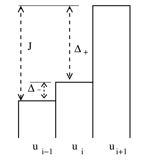
We will express a slope limiter in terms of the ratio
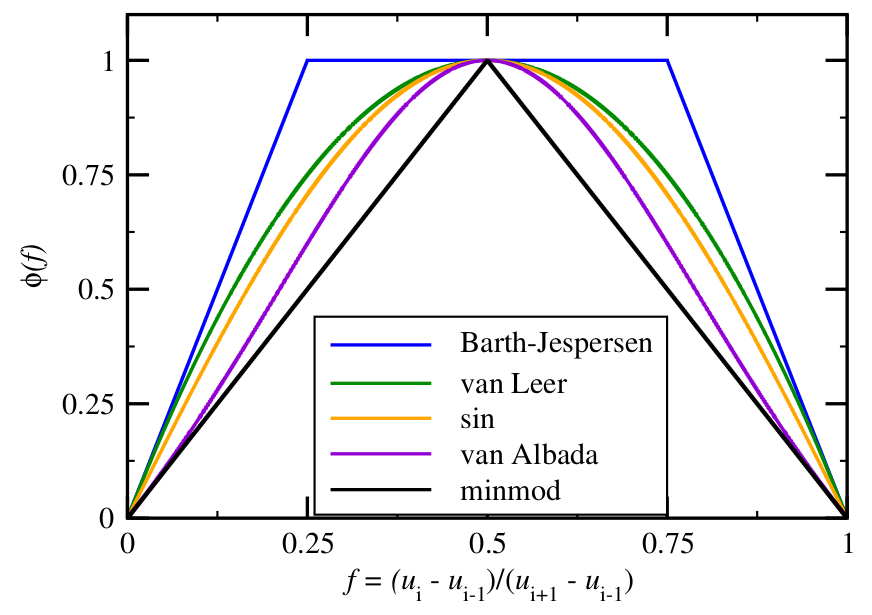 All of these limiters are second order accurate and TVD; those that fall below minmod are not second order accurate and those that are above Barth-Jesperson are not second order accurate, not TVD, or produce artifacts.
Common limiters#
limit_zero(r) = 0
limit_none(r) = 1
limit_minmod(r) = max(min(2*r, 2*(1-r)), 0)
limit_sin(r) = (0 < r && r < 1) * sinpi(r)
limit_vl(r) = max(4*r*(1-r), 0)
limit_bj(r) = max(0, min(1, 4*r, 4*(1-r)))
limiters = [limit_zero limit_none limit_minmod limit_sin limit_vl limit_bj];
plot(limiters, label=limiters, xlims=(-.1, 1.1))
A slope-limited solver#
function fv_solve2(riemann, u_init, n, tfinal=1, limit=limit_sin)
    h = 2 / n
    x = LinRange(-1+h/2, 1-h/2, n) # cell midpoints (centroids)
    idxL = 1 .+ (n-1:2*n-2) .% n
    idxR = 1 .+ (n+1:2*n) .% n
    function rhs(t, u)
        jump = u[idxR] - u[idxL]
        r = (u - u[idxL]) ./ jump
        r[isnan.(r)] .= 0
        g = limit.(r) .* jump / 2h
        fluxL = riemann(u[idxL] + g[idxL]*h/2, u - g*h/2)
        fluxR = fluxL[idxR]
        (fluxL - fluxR) / h
    end
    thist, uhist = ode_rk_explicit(
        rhs, u_init.(x), h=h, tfinal=tfinal)
    x, thist, uhist
end
fv_solve2 (generic function with 3 methods)
x, thist, uhist = fv_solve2(riemann_advection, testfunc, 200, 10,
    limit_sin)
plot(x, uhist[:,1:400:end], legend=:none)
Hyperbolic systems#
Isentropic gas dynamics#
Variable |
meaning |
|---|---|
\(\rho\) |
density |
\(u\) |
velocity |
\(\rho u\) |
momentum |
\(p\) |
pressure |
Equation of state \(p(\rho) = C \rho^\gamma\) with \(\gamma = 1.4\) (typical air).
“isothermal” gas dynamics: \(p(\rho) = c^2 \rho\), wave speed \(c\).
Compute as \( \rho u^2 = \frac{(\rho u)^2}{\rho} .\)
Smooth wave structure#
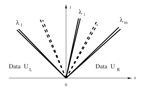
For perturbations of a constant state, systems of equations produce multiple waves with speeds equal to the eigenvalues of the flux Jacobian,
Riemann problem for systems: shocks#
Given states \(U_L\) and \(U_R\), we will see two waves with some state \(U^*\) in between. There could be two shocks, two rarefactions, or one of each. The type of wave will determine the condition that must be satisfied to connect \(U_L\) to \(U_*\) and \(U_*\) to \(U_R\).
Left-moving wave#
If there is a shock between \(U_L\) and \(U_*\), the Rankine-Hugoniot condition
Solving the first equation for \(s\) and substituting into the second, we compute \begin{split} \frac{(\rho_* u_* - \rho_L u_L)^2}{\rho_* - \rho_L} &= \rho_* u_^2 - \rho_L u_L^2 + c^2 (\rho_ - \rho_L) \ \rho_^2 u_^2 - 2 \rho_* \rho_L u_* u_L + \rho_L^2 u_L^2 &= \rho_* (\rho_* - \rho_L) u_^2 - \rho_L (\rho_ - \rho_L) u_L^2 + c^2 (\rho_* - \rho_L)^2 \ \rho_* \rho_L \Big( u_^2 - 2 u_ u_L + u_L^2 \Big) &= c^2 (\rho_* - \rho_L)^2 \ (u_* - u_L)^2 &= c^2 \frac{(\rho_* - \rho_L)^2}{\rho_* \rho_L} \ u_* - u_L &= \pm c \frac{\rho_* - \rho_L}{\sqrt{\rho_* \rho_L}} \end{split} and will need to use the entropy condition to learn which sign to take.
Admissible shocks#
We need to choose the sign
The entropy condition requires that
Right-moving wave#
The same process for the right wave \(\lambda(U) = u + c\) yields a shock when \(\rho_* \ge \rho_R\), in which case the velocity jump is
Rarefactions#
A rarefaction occurs when
Generalized Riemann invariants#
(Derivation of this condition is beyond the scope of this class.)
Isothermal gas dynamics#
across the wave \(\lambda = u-c\). We can rearrange to
Integration yields
Basic algorithm#
Find \(\rho_*\)
Use entropy condition (for shock speeds)
If it’s a shock: find \(u_*\) using Rankine-Hugoniot
If it’s a rarefaction: use generalized Riemann invariant
First a miracle happens#
In general we will need to use a Newton method to solve for the state in the star region.