2022-11-30 Reconstruction

Last time

• Notes on unstructured meshing workflow

• Finite volume methods for hyperbolic conservation laws

• Riemann solvers for scalar equations

  • Shocks and the Rankine-Hugoniot condition

  • Rarefactions and entropy solutions

Today

• Godunov’s Theorem

• Slope reconstruction and limiting

• Hyperbolic systems

  • Rankine-Hugoniot and Riemann Invariants

  • Exact Riemann solvers

  • Approximate Riemann solvers

using LinearAlgebra
using Plots
default(linewidth=3)

struct RKTable
    A::Matrix
    b::Vector
    c::Vector
    function RKTable(A, b)
        s = length(b)
        A = reshape(A, s, s)
        c = vec(sum(A, dims=2))
        new(A, b, c)
    end
end

rk4 = RKTable([0 0 0 0; .5 0 0 0; 0 .5 0 0; 0 0 1 0], [1, 2, 2, 1] / 6)

function ode_rk_explicit(f, u0; tfinal=1., h=0.1, table=rk4)
    u = copy(u0)
    t = 0.
    n, s = length(u), length(table.c)
    fY = zeros(n, s)
    thist = [t]
    uhist = [u0]
    while t < tfinal
        tnext = min(t+h, tfinal)
        h = tnext - t
        for i in 1:s
            ti = t + h * table.c[i]
            Yi = u + h * sum(fY[:,1:i-1] * table.A[i,1:i-1], dims=2)
            fY[:,i] = f(ti, Yi)
        end
        u += h * fY * table.b
        t = tnext
        push!(thist, t)
        push!(uhist, u)
    end
    thist, hcat(uhist...)
end

function testfunc(x)
    max(1 - 4*abs.(x+2/3),
        abs.(x) .< .2,
        (2*abs.(x-2/3) .< .5) * cospi(2*(x-2/3)).^2
    )
end

flux_advection(u) = u
flux_burgers(u) = u^2/2
flux_traffic(u) = u * (1 - u)

riemann_advection(uL, uR) = 1*uL # velocity is +1

function fv_solve1(riemann, u_init, n, tfinal=1)
    h = 2 / n
    x = LinRange(-1+h/2, 1-h/2, n) # cell midpoints (centroids)
    idxL = 1 .+ (n-1:2*n-2) .% n
    idxR = 1 .+ (n+1:2*n) .% n
    function rhs(t, u)
        fluxL = riemann(u[idxL], u)
        fluxR = riemann(u, u[idxR])
        (fluxL - fluxR) / h
    end
    thist, uhist = ode_rk_explicit(rhs, u_init.(x), h=h, tfinal=tfinal)
    x, thist, uhist
end

function riemann_burgers(uL, uR)
    flux = zero(uL)
    for i in 1:length(flux)
        fL = flux_burgers(uL[i])
        fR = flux_burgers(uR[i])
        flux[i] = if uL[i] > uR[i] # shock
            max(fL, fR)
        elseif uL[i] > 0 # rarefaction all to the right
            fL
        elseif uR[i] < 0 # rarefaction all to the left
            fR
        else
            0
        end
    end
    flux
end

function riemann_traffic(uL, uR)
    flux = zero(uL)
    for i in 1:length(flux)
        fL = flux_traffic(uL[i])
        fR = flux_traffic(uR[i])
        flux[i] = if uL[i] < uR[i] # shock
            min(fL, fR)
        elseif uL[i] < .5 # rarefaction all to the right
            fL
        elseif uR[i] > .5 # rarefaction all to the left
            fR
        else
            flux_traffic(.5)
        end
    end
    flux 
end

riemann_traffic (generic function with 1 method)

Godunov methods (first order accurate)

init_func(x) = testfunc(x)
x, thist, uhist = fv_solve1(riemann_traffic, init_func, 100, 2)
plot(x, uhist[:,1:5:end], legend=:none)

Burgers

• flux \(u^2/2\) has speed \(u\)

• negative values make sense

• satisfies a maximum principle

Traffic

• flux \(u - u^2\) has speed \(1 - 2u\)

• state must satisfy \(u \in [0, 1]\)

Godunov’s Theorem (1954)

Linear numerical methods

\[ \dot u_i = \sum_j a_{ij} u_j \]

for solving time-dependent PDE can be at most first order accurate if they are monotone.

For our purposes, monotonicity is equivalent to positivity preservation,

\[ \min_x u(0, x) \ge 0 \quad \Longrightarrow \quad \min_x u(t, 0) \ge 0 .\]

Discontinuities

A numerical method for representing a discontinuous function on a stationary grid can be no better than first order accurate in the \(L^1\) norm,

\[ \lVert u - u^* \rVert_{L^1} = \int \lvert u - u^* \rvert . \]

If we merely sample a discontinuous function, say

\[\begin{split} u(x) = \begin{cases} 0, & x \le a \\ 1, & x > a \end{cases} \end{split}\]

onto a grid with element size \(\Delta x\) then we will have errors of order 1 on an interval proportional to \(\Delta x\).

In light of these two observations, we may still ask for numerical methods that are more than first order accurate for smooth solutions, but those methods must be nonlinear.

Slope Reconstruction

One method for constructing higher order methods is to use the state in neighboring elements to perform a conservative reconstruction of a piecewise polynomial, then compute numerical fluxes by solving Riemann problems at the interfaces. If \(x_i\) is the center of cell \(i\) and \(g_i\) is the reconstructed gradient inside cell \(i\), our reconstructed solution is

\[ \tilde u_i(x) = u_i + g_i \cdot (x - x_i) . \]

We would like this reconstruction to be monotone in the sense that

\[ \Big(\tilde u_i(x) - \tilde u_j(x) \Big) \Big( u_i - u_j \Big) \ge 0 \]

for any \(x\) on the interface between element \(i\) and element \(j\).

Question

Is the symmetric slope

\[ \hat g_i = \frac{u_{i+1} - u_{i-1}}{2 \Delta x} \]

monotone?

Slope limiting

We will determine gradients by “limiting” the above slope using a nonlinear function that reduces to 1 when the solution is smooth. There are many ways to express limiters and our discussion here roughly follows Berger, Aftosmis, and Murman (2005).

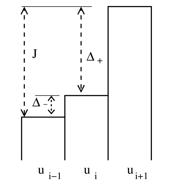
We will express a slope limiter in terms of the ratio

\[ r_i = \frac{u_i - u_{i-1}}{u_{i+1} - u_{i-1}} \]

and use as a gradient,

\[ g_i = \phi(r_i) \frac{u_{i+1} - u_{i-1}}{2 \Delta x} . \]

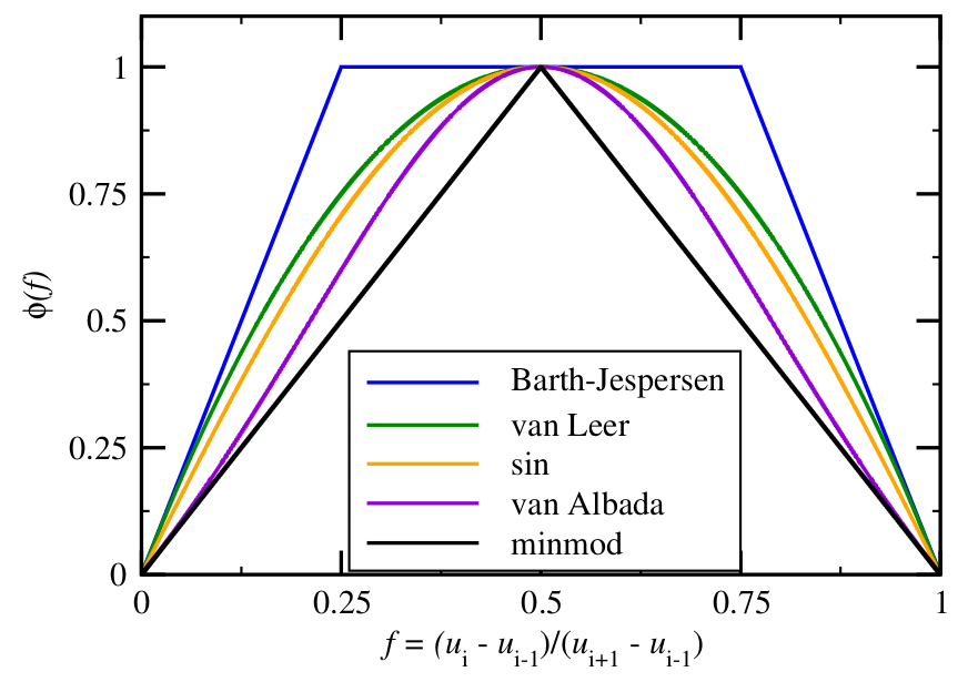Our functions \(\phi\) will be zero unless \(0 < r < 1\) and \(\phi(1/2) = 1\). All of these limiters are second order accurate and TVD; those that fall below minmod are not second order accurate and those that are above Barth-Jesperson are not second order accurate, not TVD, or produce artifacts.

Common limiters

limit_zero(r) = 0
limit_none(r) = 1
limit_minmod(r) = max(min(2*r, 2*(1-r)), 0)
limit_sin(r) = (0 < r && r < 1) * sinpi(r)
limit_vl(r) = max(4*r*(1-r), 0)
limit_bj(r) = max(0, min(1, 4*r, 4*(1-r)))
limiters = [limit_zero limit_none limit_minmod limit_sin limit_vl limit_bj];

plot(limiters, label=limiters, xlims=(-.1, 1.1))

A slope-limited solver

function fv_solve2(riemann, u_init, n, tfinal=1, limit=limit_sin)
    h = 2 / n
    x = LinRange(-1+h/2, 1-h/2, n) # cell midpoints (centroids)
    idxL = 1 .+ (n-1:2*n-2) .% n
    idxR = 1 .+ (n+1:2*n) .% n
    function rhs(t, u)
        jump = u[idxR] - u[idxL]
        r = (u - u[idxL]) ./ jump
        r[isnan.(r)] .= 0
        g = limit.(r) .* jump / 2h
        fluxL = riemann(u[idxL] + g[idxL]*h/2, u - g*h/2)
        fluxR = fluxL[idxR]
        (fluxL - fluxR) / h
    end
    thist, uhist = ode_rk_explicit(
        rhs, u_init.(x), h=h, tfinal=tfinal)
    x, thist, uhist
end

fv_solve2 (generic function with 3 methods)

x, thist, uhist = fv_solve2(riemann_advection, testfunc, 100, .5,
    limit_sin)
plot(x, uhist[:,1:10:end], legend=:none)

Hyperbolic systems

\[ U_t + f(U)_x = 0 \]

Isentropic gas dynamics

(65)\[\begin{align} U &= \begin{bmatrix} \rho \\ \rho u \end{bmatrix} & f(U) &= \begin{bmatrix} \rho u \\ \rho u^2 + p \end{bmatrix} \end{align}\]

Variable	meaning
\(\rho\)	density
\(u\)	velocity
\(\rho u\)	momentum
\(p\)	pressure

• Equation of state \(p(\rho) = C \rho^\gamma\) with \(\gamma = 1.4\) (typical air).

• “isothermal” gas dynamics: \(p(\rho) = c^2 \rho\), wave speed \(c\).

• Compute as \( \rho u^2 = \frac{(\rho u)^2}{\rho} .\)

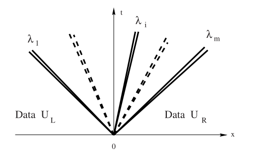
Smooth wave structure

For perturbations of a constant state, systems of equations produce multiple waves with speeds equal to the eigenvalues of the flux Jacobian,

\[\begin{split} f'(U) = \begin{bmatrix} 0 & 1 \\ -u^2 + c^2 & 2 u \end{bmatrix}. \end{split}\]

We can compute the eigenvalues and eigenvectors,

\[ f'(U) = W \Lambda W^{-1} \]

as

(66)\[\begin{align} W &= \begin{bmatrix} 1 & 1 \\ u-c & u+c \end{bmatrix} & \Lambda &= \begin{bmatrix} u-c & \\ & u+c \end{bmatrix} . \end{align}\]

Riemann problem for systems: shocks

Given states \(U_L\) and \(U_R\), we will see two waves with some state \(U^*\) in between. There could be two shocks, two rarefactions, or one of each. The type of wave will determine the condition that must be satisfied to connect \(U_L\) to \(U_*\) and \(U_*\) to \(U_R\).

Left-moving wave

If there is a shock between \(U_L\) and \(U_*\), the Rankine-Hugoniot condition

\[ s \Delta U = \Delta f \]

will be satisfied along with the entropy condition

\[ \lambda_i(U_L) \ge s \ge \lambda_i(U_*) \]

where \(\lambda_i(U)\) is the corresponding eigenvalue of the flux Jacobian \(f'(U)\). The inequality in the entropy condition is strict if the wave is genuinely nonlinear. For isothermal gas dynamics, the Rankine-Hugoniot condition is

(67)\[\begin{align} (\rho_* - \rho_L) s &= \rho_* u_* - \rho_L u_L \\ (\rho_* u_* - \rho_L u_L) s &= \Big(\rho_* u_*^2 + c^2 \rho_* \Big) - \Big( \rho_L u_L^2 + c^2 \rho_L \Big) \end{align}\]

Solving the first equation for \(s\) and substituting into the second, we compute \begin{split} \frac{(\rho_* u_* - \rho_L u_L)^2}{\rho_* - \rho_L} &= \rho_* u_^2 - \rho_L u_L^2 + c^2 (\rho_ - \rho_L) \ \rho_^2 u_^2 - 2 \rho_* \rho_L u_* u_L + \rho_L^2 u_L^2 &= \rho_* (\rho_* - \rho_L) u_^2 - \rho_L (\rho_ - \rho_L) u_L^2 + c^2 (\rho_* - \rho_L)^2 \ \rho_* \rho_L \Big( u_^2 - 2 u_ u_L + u_L^2 \Big) &= c^2 (\rho_* - \rho_L)^2 \ (u_* - u_L)^2 &= c^2 \frac{(\rho_* - \rho_L)^2}{\rho_* \rho_L} \ u_* - u_L &= \pm c \frac{\rho_* - \rho_L}{\sqrt{\rho_* \rho_L}} \end{split} and will need to use the entropy condition to learn which sign to take.

Admissible shocks

We need to choose the sign

\[u_* - u_L = \pm c \frac{\rho_* - \rho_L}{\sqrt{\rho_*\rho_L}}\]

The entropy condition requires that

\[ \lambda(U_L) = u_L - c \ge s \ge u_* - c = \lambda(U_*) . \]

Meanwhile, the first Rankine-Hugoniot condition and \(\rho > 0\) provides

\[ \rho_L c \le \rho_L (u_L - s) = \rho_* (u_* - s) \le \rho_* c \]

which is to say that \(\rho_* \ge \rho_L\) and consequently we take the negative sign,

\[ u_* - u_L = - c\frac{\rho_* - \rho_L}{\sqrt{\rho_* \rho_L}} .\]

Right-moving wave

The same process for the right wave \(\lambda(U) = u + c\) yields a shock when \(\rho_* \ge \rho_R\), in which case the velocity jump is

\[ u_R - u_* = - c \frac{\rho_* - \rho_R}{\sqrt{\rho_* \rho_R}} . \]

Rarefactions

A rarefaction occurs when

\[ \lambda_i(U_L) < \lambda_i(U_R) \]

Generalized Riemann invariants

\[ \frac{d U^1}{W_i^1} = \frac{d U^2}{W_i^2} = \dotsb \]

(Derivation of this condition is beyond the scope of this class.)

Isothermal gas dynamics

\[ \frac{d \rho}{1} = \frac{d (\rho u)}{u - c} \]

across the wave \(\lambda = u-c\). We can rearrange to

\[ (u-c) d \rho = \rho d u + u d \rho \]

or

\[ d u + \frac{c}{\rho} d \rho = 0 . \]

Integration yields

\[ u + \int \frac{c}{\rho} d \rho = u + c \log \rho = \text{constant} . \]

So if we have a rarefaction between \(U_L\) and \(U_*\) then

\[ u_L + c \log \rho_L = u_* + c \log \rho_* . \]

Similarly, for the wave \(\lambda = u + c\), a rarefaction between \(U_*\) and \(U_R\) results in

\[ u_* - c \log \rho_* = u_R - c \log \rho_R . \]

If the rarefaction is sonic, we have \(u_0 - c = 0\) for a left rarefaction (or \(u_0 + c =0\) for the right) and can compute \(\rho_0\) from

\[ u_* -c \log \rho_* = u_0 - c \log \rho_0,\]

via

\[ \rho_0 = \exp\big[(u_0 - u_*)/c + \log \rho_* \big].\]

Basic algorithm

1. Find \(\rho_*\)

2. Use entropy condition (for shock speeds)

• If it’s a shock: find \(u_*\) using Rankine-Hugoniot

• If it’s a rarefaction: use generalized Riemann invariant

First a miracle happens

In general we will need to use a Newton method to solve for the state in the star region.

Exact Riemann solver for isothermal gas dynamics

function flux_isogas(U, c=1)
    rho = U[1]
    u = U[2] / rho
    [U[1], U[1]*u + c^2*rho]
end

function ujump_isogas(rho_L, rho_R, c=1)
    if rho_R > rho_L # shock
        (rho_L - rho_R) / sqrt(rho_L*rho_R)
    else # rarefaction
        c * (log(rho_L) - log(rho_R))
    end
end

function dujump_isogas(rho_L, drho_L, rho_R, drho_R, c=1)
    if rho_R > rho_L # shock
        ((drho_L - drho_R) / sqrt(rho_L*rho_R)
            - .5*(rho_L - rho_R) * (rho_L*rho_R)^(-3/2) * (drho_L * rho_R + rho_L * drho_R))
    else
        c * (drho_L / rho_L - drho_R / rho_R)
    end
end

dujump_isogas (generic function with 2 methods)

function riemann_isogas(UL, UR, maxit=20)
    rho_L, u_L = UL[1], UL[2]/UL[1]
    rho_R, u_R = UR[1], UR[2]/UR[1]
    rho = .5 * (rho_L + rho_R) # initial guess
    for i in 1:maxit
        f = (ujump_isogas(UL[1], rho)
            + ujump_isogas(rho, UR[1])
            - (UR[2]/UR[1] - UL[2]/UL[1]))
        if norm(resid) < 1e-10
            u = u_L + ujump_isogas(UL[1], rho)
            break
        end
        J = (dujump_isogas(UL[1], 0, rho, 1)
            + dujump_isogas(rho, 1, uR[1], 0))
        delta_rho = -f / J
        while min(rho + delta_rho <= 0)
            delta_rho /= 2 # line search to prevent negative rho
        end
    end
    U0 = resolve_isogas(UL, UR, rho)
    flux_isogas(U0)
end

riemann_isogas (generic function with 2 methods)

Resolving waves for isothermal gas dynamics

function resolve_isogas(UL, UR, U_star)
    rho_L, u_L = UL[1], UL[2]/UL[1]
    rho_R, u_R = UR[1], UR[2]/UR[1]
    rho, u = U_star[1], U_star[2] / U_star[1]
    if u_L - c < 0 < u - c || u + c < 0 < u_R + c
        # inside left (right) sonic rarefaction
        u0 = sign(u) * c
        rho0 = exp((u0-u)/c + log(rho))
        return [rho0, rho0 * u0]
    elseif ((rho_L >= rho && 0 <= u_L - c) ||
            (rho_L < rho && 0 < rho*u - UL[2]))
        return UL
    elseif ((rho_R >= rho && u_R + c <= 0) ||
            (rho_R < rho && UR[2] - rho*u > 0))
        return UR
    end
    [rho, rho*u]
end

resolve_isogas (generic function with 1 method)

function initial_isogas(x)
    [1 .+ 2 * exp.(-4x .^ 2) 0*x]
end

x = LinRange(-1, 1, 100)
U = initial_isogas(x)
plot(x, U)

Solver

function fv_solve2system(riemann, u_init, n, tfinal=1, limit=limit_sin)
    h = 2 / n
    x = LinRange(-1+h/2, 1-h/2, n) # cell midpoints (centroids)
    idxL = 1 .+ (n-1:2*n-2) .% n
    idxR = 1 .+ (n+1:2*n) .% n
    U0 = u_init(x)
    m, n = size(U0)
    @show size(U0)
    function rhs(t, U)
        U = reshape(U, m, n)
        jump = u[:,idxR] - u[:,idxL]
        r = (u - u[idxL]) ./ jump
        r[isnan.(r)] .= 0
        g = limit.(r) .* jump / 2h
        fluxL = riemann(u[idxL] + g[idxL]*h/2, u - g*h/2)
        fluxR = fluxL[idxR]
        (fluxL - fluxR) / h
    end
    thist, uhist = ode_rk_explicit(
        rhs, u_init.(x), h=h, tfinal=tfinal)
    x, thist, uhist
end

fv_solve2system (generic function with 3 methods)

x, t_hist, U_hist = fv_solve2system(riemann_isogas, initial_isogas, 100, 0.1)
size(U_hist)

size(U0) = (100, 2)

MethodError: no method matching +(::Matrix{Float64}, ::Float64)
For element-wise addition, use broadcasting with dot syntax: array .+ scalar
Closest candidates are:
  +(::Any, ::Any, ::Any, ::Any...) at operators.jl:591
  +(::T, ::T) where T<:Union{Float16, Float32, Float64} at float.jl:383
  +(::AbstractArray, ::StaticArraysCore.StaticArray) at ~/.julia/packages/StaticArrays/6QFsp/src/linalg.jl:13
  ...

Stacktrace:
  [1] _broadcast_getindex_evalf
    @ ./broadcast.jl:670 [inlined]
  [2] _broadcast_getindex
    @ ./broadcast.jl:643 [inlined]
  [3] getindex
    @ ./broadcast.jl:597 [inlined]
  [4] copy
    @ ./broadcast.jl:899 [inlined]
  [5] materialize
    @ ./broadcast.jl:860 [inlined]
  [6] broadcast_preserving_zero_d
    @ ./broadcast.jl:849 [inlined]
  [7] +(A::Vector{Matrix{Float64}}, Bs::Vector{Float64})
    @ Base ./arraymath.jl:16
  [8] ode_rk_explicit(f::var"#rhs#4"{typeof(riemann_isogas), Int64, typeof(limit_sin), Int64, Vector{Int64}, Vector{Int64}, Float64}, u0::Vector{Matrix{Float64}}; tfinal::Float64, h::Float64, table::RKTable)
    @ Main ./In[1]:31
  [9] fv_solve2system(riemann::typeof(riemann_isogas), u_init::typeof(initial_isogas), n::Int64, tfinal::Float64, limit::Function)
    @ Main ./In[11]:19
 [10] fv_solve2system(riemann::Function, u_init::Function, n::Int64, tfinal::Float64)
    @ Main ./In[11]:2
 [11] top-level scope
    @ In[12]:1
 [12] eval
    @ ./boot.jl:368 [inlined]
 [13] include_string(mapexpr::typeof(REPL.softscope), mod::Module, code::String, filename::String)
    @ Base ./loading.jl:1428

Approximate Riemann solvers

Exact Riemann solvers are

• complicated to implement

• fragile in the sense that small changes to the physics, such as in the equation of state \(p(\rho)\), can require changing many conditionals

• the need to solve for \(\rho^*\) using a Newton method and then evaluate each case of the wave structure can be expensive.

• An exact Riemann solver has never been implemented for some equations.

HLL (Harten, Lax, and van Leer)

Assume two shocks with speeds \(s_L\) and \(s_R\). These speeds will be estimated and must be at least as fast as the fastest left- and right-traveling waves. If the wave speeds \(s_L\) and \(s_R\) are given, we have the Rankine-Hugoniot conditions across both shocks,

(68)\[\begin{align} s_L (U_* - U_L) &= f(U_*) - f(U_L) \\ s_R (U_R - U_*) &= f(U_R) - f(U_*) . \end{align}\]

Adding these together gives

\[s_R U_R - (s_R - s_L) U_* - s_L U_L = f(U_R) - f(U_L)\]

which can be solved for \(U_*\) as

\[ U_* = \frac{f(U_L) - f(U_R) - s_L U_L + s_R U_R}{s_R - s_L} . \]

We can save an extra evaluation of the flux by using the Rankine-Hugoniot conditions

\[ f(U_*) = \frac{s_R f(U_L) - s_L f(U_R) + s_L s_R (U_R - U_L)}{s_R - s_L} . \]

Isothermal gas dynamics

(69)\[\begin{align} s_L &= \min( u_L - c, u_R - c ) \\ s_R &= \max(u_L + c, u_R + c) \end{align}\]

Rusanov method

Special case \(s_L = - s_R\), in which case the wave structure is always subsonic and the flux is simply

\[f(U_*) = \frac 1 2 \Big( f(U_L) + f(U_R) \Big) - \frac s 2 \Big( U_R - U_L \Big) . \]

Observations on HLL solvers

\[ f(U_*) = \frac{s_R f(U_L) - s_L f(U_R) + s_L s_R (U_R - U_L)}{s_R - s_L} . \]

• The term involving \(U_R-U_L\) represents diffusion and will cause entropy to decay (physical entropy is produced).

• If our Riemann problem produces shocks and we have correctly calculated the wave speeds, the HLL solver is exact and produces the minimum diffusion necessary for conservation.

• If the wave speed estimates are slower than reality, the method will be unstable due to CFL.

• If the wave speed estimates are faster than reality, the method will be more diffusive than an exact Riemann solver.